Silent Sound Demo schematics, circuit and operational theory documents

The following is extracted from “the Silent Sound Demo for the mind control machinery”. This come from the time (around 2000) when the patent was first granted and the inventor was trying to sell his device. It is extracted from historical archives and is useful in helping us design our own systems to conduct affirmations prayer campaigns.

This entire article lists the schematics, parts list and construction blueprints of a demo device that shows the principles of the Silent Sound Technology that is now in use by almost all of the United States government agencies, the mainstream media and advertisement companies.

This is for those who want to DIY their own system, or who want to experiment themselves. I am afraid that it is a bit technical, but I am a geek and this kind of stuff excites me so much.

It’s like a pretty girl wearing an awesome dress (with cute earrings, and a really nice set of high heels), some tasty shraz wine, and a super delicious pizza all together for a night of magic.

But that’s just me. I am such a sucker for a girl wearing a dress, high heels and really cute earrings. Not to mention pizza and shraz wine.

For those of you who are not geeks, please just skim the article and realize that it exists. Future articles will build upon the information provided here and make it very easy to hack into your own brain and biological systems so that YOU have control over your body and your MWI.

Great stuff actually. But sorry for the technical opacification.

The Schematic

Here’s a nice overview summary of the circuit schematic. Obviously, it is not an overly complex device; Four IC chips, a handful of capacitors and resistors and a transistor.
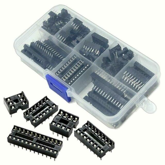
Silent Sound Demo schematic

Use Chip Sockets

Do not go all in for hard-wiring and soldering everything. Use male and female connectors and attach using this convention. And Lordy, please refrain from wire wrapping.

An IC socket, also known as a chip socket, or a DIP IC socket is an electrical connector used in the field of electronic engineer. The pins of the integrated circuit (IC) connect into the socket making a robust electrical connection without the requirement of soldering.

-DIP IC Sockets - Peter Vis
Examples of various sizes of chip sockets.

The Drawings

The several Corel Draw 3 .CDR drawings referenced below will NOT display in most browsers. The idea is that you SAVE TO YOUR LOCAL HARD DRIVE each one, then print from a compatible graphics package. This method gives the clearest quality prints.
I HAVE ALSO INCLUDED .GIF DRAWINGS, HOWEVER, DUE TO THE COARSE RESOLUTION OF MY GRAPHICS SOFTWARE, THESE MAY OR MAY NOT PRINT TO MEET YOUR NEEDS.
An office services shop should be able to print the .CDRs – BE SURE THEY SELECT “FIT TO PAGE”. (Note that this instruction packet is dated from 2001. – MM) Most recent full featured graphics packages can read and print a Corel Draw 3 (VECTOR) drawing. The entire set of .CDR files will fit on one EMPTY 1.44 MB floppy diskette. (Thus dating this article. LOL.) Here are the clickable references, sizes, and paper orientation.

The Documents for the Large Version

The Documents for the Small Version

SMALLER PERF BOARD VERSION – NO BOARD CUTTING REQUIRED ** >> DRAWINGS ABOVE ARE SUFFICIENT FOR SOMEONE WHO CAN DESIGN THEIR OWN CASE AND PANEL

Questions and Answers

Q: Are the items in question expensive? I MIGHT be interested in paying for a demo unit. How large and heavy is it when finished
.
A: I estimate it could be done for about $200 US (year 2000 prices), though this would vary upwards if you had to purchase a tape recorder, say, or a frequency meter along with it. Tape recorder, a small one, is necessary. A frequency meter is not, subject to conditions below. With the largest Radio Shack plastic project box, it’s 8″ x 6″ x 3″. With the 12-volt gel cell inside, it weighs perhaps 3 lbs.
.
Q: Could you briefly describe how you demo it to curious onlookers?
.
A: I keep a tape recorder with sample ordinary voice with the unit, so I can demonstrate both the 1,500 Hertz normal speech center freq. then raise the center frequency up until it is not audible. At that point, the visitor is hearing “silent sound” carrying speech, using FM rather than nature’s AM.
.
I also unplug the attenuator / patch cable from the “earphone” jack on the tape recorder, which allows the visitor to hear the ordinary voice on the tape, which is AM (amplitude modulation). Also at that point, the brain is using “slope tuning” to recover the normal voice from the inaudible signal.
.
I tell them this is an unclassified device which can hypontize SILENTLY, show them the label with the U.S. patent #5,159,703, and tell them a unit like this was used in the 1991 Gulf War by the U.S. Army Psychological Warfare branch to persuade, silently, all those Iraqi troops to surrender so quickly.
.
That was DOCUMENTED on ITV, and you should have for your reference (one copy, not to hand out – it’s too long) the Judy Wall article at this link: http://www.raven1.net/silsoun2.htm.
.
I go on to tell them that this device gets it’s REAL destructive power when connected to a voice to skull transmitter, one of which is under construction here in Ontario. It can beam hypnosis silently into someone’s skull for years and they won’t be aware.
.
Q: Can you monitor the output?
.
A: You CAN use the Radio Shack sound level meter to show, when the frequency setting is high, that sound is coming out of the tweeter even though they can’t hear it. Due to having to use the bus, I’m restricted on how much I can carry, so I haven’t used this but once. (Doesn’t seem to be required, actually.) However, there are a couple of important caveats if you want to use a sound level meter:

.

  • Radio Shack’s sound level meters are calibrated to match the human ear response.
  • Since the demo unit can easily tune the center frequency up above 20 kHz (the meter’s upper limit) you must have a FREQUENCY COUNTER with you or your sound level meter may miss your then-ultrasound signal.
  • This demo unit, in order to pump out any kind of signal near the high end of human hearing (around 15 kHz) uses a small PIEZO tweeter, 2 inches dia.
  • The readily available, simple, LM386 audio amplifier chip will handle this frequency, but without much power to spare, so the actual amplitude is not great at 14.5 kHz, the Lowery patent specification.
  • Therefore, especially OUTDOORS, a demo to use a sound level meter needs an ADDITIONAL STAGE of amplification. That could be added on to the circuit board, but room is a problem with the 276-158 board, or, an amplified speaker, like the Radio Shack 21-541 would be needed for a reliably convincing sound level meter demo. (The 21-541 should also have it’s low-frequency speaker replaced with a 30,000 Hz PIEZO tweeter.)
The GOOD news is that so far, the sound level meter demo does NOT seem to be necessary, though I do have the equipment should that be necessary. The full demo would probably be used for a pre-arranged meeting with a group.

Demonstration Spiel for Silent Sound Demo Device September 28, 2000

DEMONSTRATION PROCEDURES THOROUGHLY go through the setup procedures first. You need to be completely familiar with the unit before attempting to demonstrate it to the public. Be sure your battery has been charged overnight.

Setup procedures Shortly before the demo, refresh yourself on: – U.S. Govt (NSA) admission mind control exists nsa1.gif – unclassified and commercial mind-weapons-capable devices uncom.htm – MKULTRA and the successful lawsuit against the CIA anat-1.htm

MATERIALS.

You need, when dealing with the public:

  • A printout of THIS SET OF INSTRUCTIONS
  • A printout of hypno2s.gif (see other below)
  • A printout of mkcover.gif (OPTIONAL)
  • ! picket sign (if outdoors without a pre-arranged meeting with visitors)
  • Some handouts, one sheet of which MUST be nsa1.gif (This has proven very compelling to those who read it)
  • For YOUR reference, a printout of Judy Wall’s article on silent sound, including Gulf War use, silsoun2.htm
  • ! copy of these instructions and spiel script
  • A small flip-nozzle container of water for your voice and perhaps throat lozenges
  • Sunscreen and sun hat if outdoors
  • A small tape recorder with a voice-ONLY cassette, normal sound
  • A patch cord between the “ear” jack on the recorder and the MONO 1/8″ jack on the demo unit (keep volume low or use an attenuator from Radio Shack. Excess volume results in garble.)

Some may find this image explaining silent sound WITHOUT the extra clutter from the voice-to-skull attachment easier to use:

  • A printout of voicefm.gif (OPTIONAL) Some may wish to hand out schematics. I recommend this schematic and matching solder-side component placement image:
  • vfmckt3.gif, schematic
  • kitbotm3.gif, solder-side layout

Components

Here’s some info on the components. And forgive me, but I am fundamentally a geek at heart.

LM386

This is a standard part.


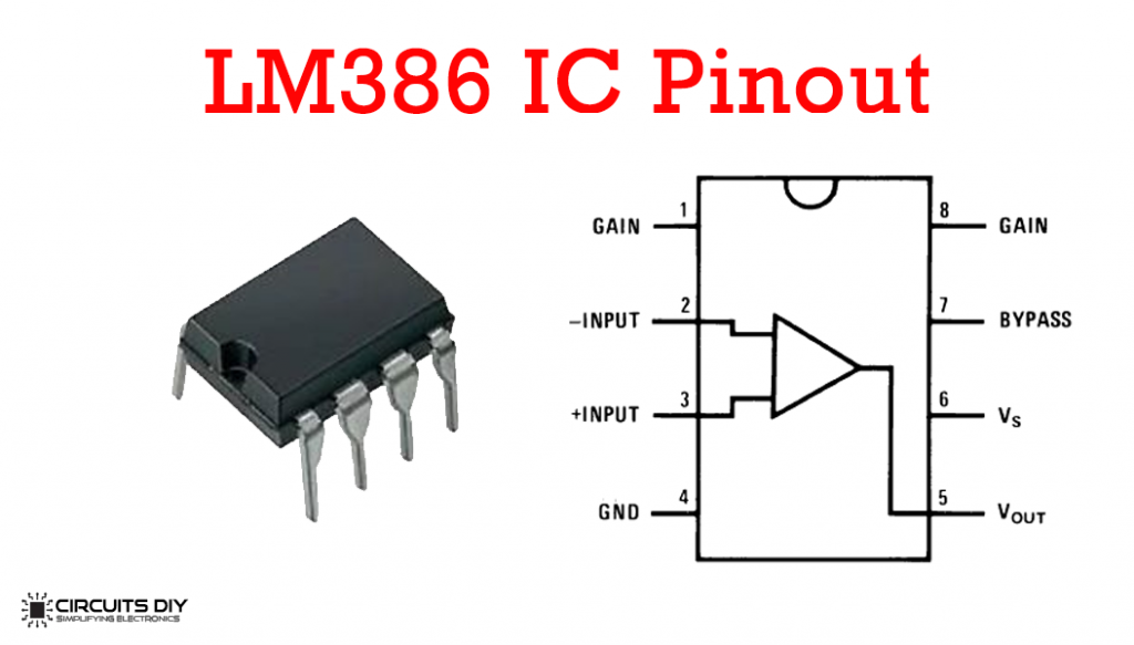
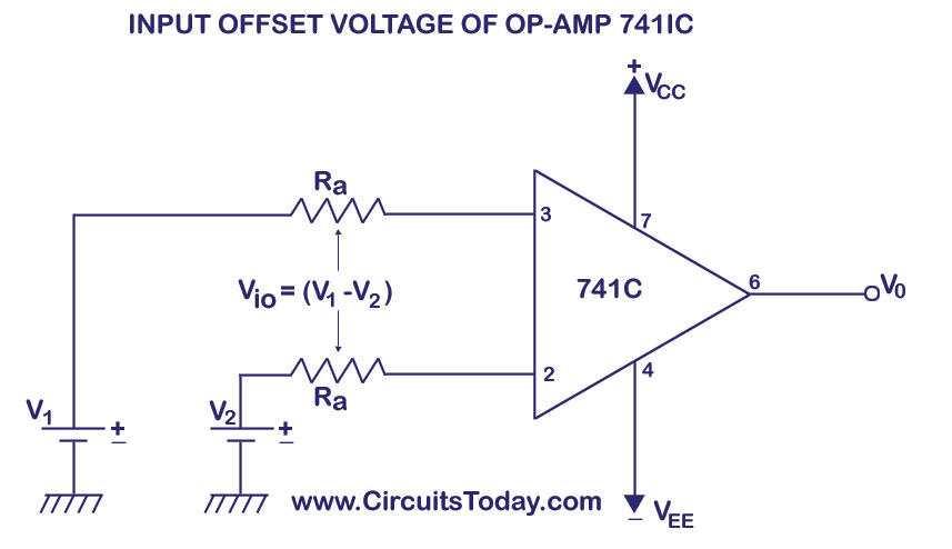
And here's another pinout.

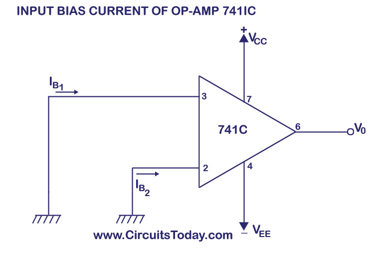
Lot's more in the PDF.

XR2206

This is a well known, if not standard, part.
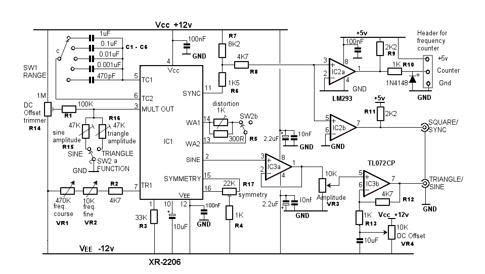
Of course, there are complete modules that you can buy that makes construction of the units so much easier. Such as this one…
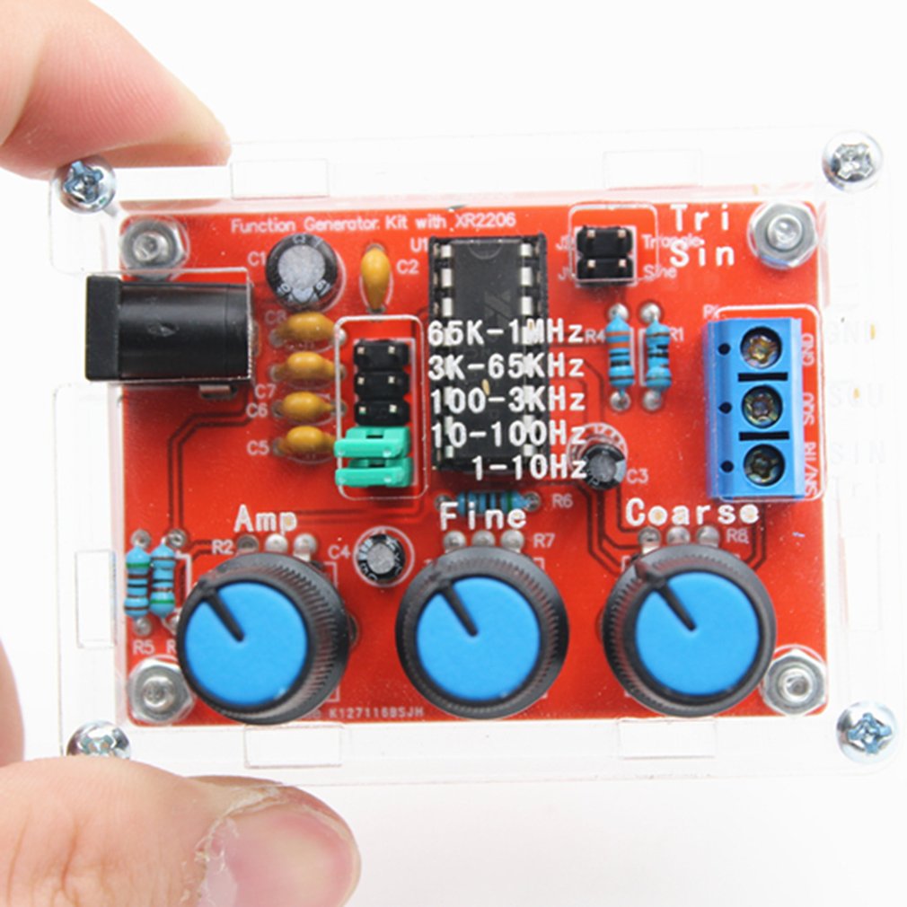
 

ICE-BREAKER.

Mine is a picket sign that carries this message: “GOVT-MEDIA TELL THE PUBLIC ABOUT ELECTRONIC MIND WEAPONS” poster9.gif

SPIEL.

The words below VARY according to the person I’m talking with, and for best effectiveness you will need to judge just how interested the visitor is. I’ve had SHORT visits like:

VISITOR: What is this? (Pointing to the demo unit)

DEMONSTRATOR: This is a device which takes ordinary human speaking voice and does two things to it: – converts it from natural AM (amplitude modulation) to FM (frequency modulation); this garbles the voice – raises the average frequency from around 1,500 Hertz, which is normal, to around 15,000 Hertz.

At 15,000 Hertz, young people with good hearing can hear a slight “ringing in the ears” from this device, while many adults hear nothing at all. But the brain CAN HEAR THE WORDS, even though the ear cannot.

This allows a hypnotist to program an individual over months and years without the target being aware. There is no resistance to the hypnosis because the target doesn’t hear it.

This can be beneficial, but it can also do severe damage to a person’s well being. This is why our group is out here demonstrating. We want government to earn their salaries and perks by placing controls on who can possess such devices and what can be legally done with them.

VISITOR: Thank you (and leaves.) LONG visits start out as above. If questions keep coming, you will need to answer them. Below are some typical questions and answers:

DEMONSTRATOR: (Continuing from the “short” spiel above) ** AT THIS POINT, YOU MAY WANT TO DROP DOWN THIS SCRIPT TO ITEM #6, THE ACTUAL PHYSICAL DEMO OF THE UNIT. I HAVE FOUND THAT A GREAT MANY VISITORS DO NOT WANT TO HEAR THE UNIT. I NEVER PRESS THAT ISSUE WITH THEM, AND ONLY START IT UP WHEN ASKED.

This device as it is here is harmless, unless used on someone who has already been programmed with trigger words or phrases. It becomes very invasive and dangerous, though, if connected to a voice-to-skull projector.

A voice-to-skull projector is a modified radar transmitter in which the human voice controls how close together the radar pulses occur.

In 1974, Dr. Joseph Sharp, of the Walter Reed Army Institute of research, announced his successful transmission of speech directly into the human skull with no receiving device.

By connecting this “silent sound” device to a voice-to-skull transmitter, it is possible to transmit hypnotic phrases silently into a target’s bedroom, every night, for years, without the target’s being aware.

By programming enough “Pavlovian triggers” into an individual, that individual’s personality can be changed substantially. Using pre-programmed trigger phrases, a “handler” of that individual can literally use him or her as a “living robot”, in cases where the individual has high susceptibility to hypnosis.

The process of programming enough triggers into an individual for purposes of control is called “creating a Manchurian Candidate”, after two books of that title. The formal program of the CIA, begun in the 1950s, started out as 149 separate experiments, and was in response to cold war fears and the apparent “brainwashing” of Allied POWs in Korea. This group of “behavior modification” experiments bore the code name MKULTRA.

MKULTRA did include electronic mind control devices, but the best known electronic mind control device of the early days was the Russian LIDA machine. The LIDA, one of which is in possession of Veterans’ Administration researcher Dr. Ross Adey, “entrained” or electronically coerced a target in the path of it’s signal to be relaxed and more susceptible to hypnosis.

A few Korean War vets claimed to have seen the LIDA in use at the POW camps. The MKULTRA code name ceased in the late 1970s when the U.S. Senate’s Frank Church Committee investigated MKULTRA experiments and found that serious atrocities had been committed on people in the military, prisons, or in mental hospitals.

However, not one single perpetrator from the MKULTRA programs was ever brought up on charges. We know that electronic mind control experimentation did not cease, and this “silent sound” technology was used in actual military combat in the 1991 Gulf War.

The United States Army connected a silent sound voice converter like this one to an FM broadcast transmitter, broadcasting on a frequency of 100 Megahertz, and the silent hypnotic commands were carried right on top of normal voice in the Iraqi language.

The normal voice carried confusing information, while the SILENT component re-inforced a sense of despair by hypnotic suggestion. This was documented on Britain’s ITV network, but not shown in the U.S. or Canada.

The successful use by the U.S. Army clearly shows that this technology does work. Through-the-wall voice-to-skull technology makes it almost inescapable.

Our group hopes that eventually the public will learn enough about the invasive privacy destroying electronic mind control weapons available today to demand that government report on these devices to the people, and make their use and possession matters of ongoing PUBLIC record.

Electronic mind control devices have been under development for 50 years, and our group knows only the unclassified and commercial versions. The time for public input and control of all such technologies is LONG overdue.

ACTUAL DEMONSTRATION OF THE UNIT ITSELF.

Put a tape with VOICE (not music) into your demo tape recorder. Connect a patch cable between the “ear” jack on the recorder and the INPUT jack on the demo unit. If you have an attenuator, use it, but if not, remember to keep the volume setting on the recorder quite low.

Excess volume garbles the speech making for an un- convincing demo. Switch on the demo unit. Adjust the tone near the lower end of the frequency knob’s travel.

The Input Level should be around one third of it’s way up from it’s lowest position.

Push PLAY on the recorder. You should hear speech “mixed” in with the demo unit’s tone.

This demonstrates to a visitor what simply converting natural human voice, which is AM or amplitude modulation to FM or frequency modulation sounds like.

Near the low end of the frequency knob’s travel, the frequencies of the voice are still about at their natural values, but the mode is now FM, as opposed to AM.

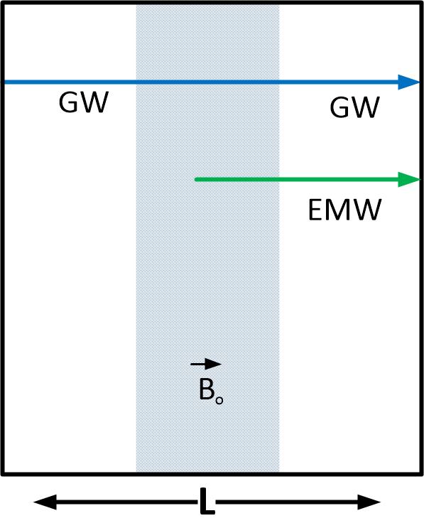
THE VISITOR CAN HEAR THIS IS GARBLED. Now slowly increase the frequency knob until the audible sound is as HIGH as you and your visitor can just hear. If you are both adults, this point is approximately where the brain can start to convert this inaudible sound BACK TO WORDS.

The process is called “slope tuning”.

You can move the IN-OFF-OUT switch back to IN to show the visitor that voice is actually being fed into the unit. vfmslopd.gif, shows how the brain recovers the inaudible words using the process of “slope detection” or “slope tuning” – worth having a few of these for technical folks who are interested in how it works.

If you have a frequency counter or meter, connect it to the two binding posts, one red, one black, on the front panel.

During a demo adjust frequency somewhere between 14.5 and 14.8 kHz (14,500 Hertz to 14,800 Hertz.) This is the range where both the Lowery patent (5,159,703) and the New Zealand Altered States company operate at to produce brain-understandable silent sound.

SEE ITEM 4 BELOW UNDER SETUP FOR COMMENTS ABOUT USING AN AUDIO LEVEL METER TO ENHANCE YOUR DEMONSTRATION.

SETUP PROCEDURES

vfmtest.gif, shows what the scope trace should look like when proper frequency modulation by voice is applied. vfmslopd.gif, shows how the brain recovers the inaudible words using the process of “slope detection” or “slope tuning” – worth having a few of these for technical folks who are interested in how it works.

1

You will need a small voltmeter to monitor battery charge state. This must be a small meter that reads out VOLTS, and *NOT* a “battery OK” meter with red and green scales.

It is necessary to know voltages for communications by email or phone with people who can offer technical help.

A convenient meter is the Radio Shack 22-802, for around $30, which has a folding case fully containing the two probes and their cable.

The only trick with any meter is TO REMEMBER TO SHUT IT OFF WHEN YOU ARE FINISHED. Almost all of today’s voltmeters have digital displays and have their own small internal battery. (Pick up and carry a spare battery.)

2

First job is to charge the internal 12-volt gel cell. The charger supplied with units purchased from Eleanor White is a simple “wall mount” style 12-volt power supply, with a cable that cannot be connected with the wrong polarity.

Measure the voltage by touching the positive (red lead) screw on the terminal strip with the red probe, and the negative (black lead) screw on the terminal strip with the black probe.

You should get “13 something” volts if the battery is reasonably well charged. If you get zero volts, it is likely that one of the 3/4 amp fuses is blown.

Check both fuses to be sure. (You can check a fuse visually, but 3/4 amp size is hard to see. Instead, switch your meter to K-ohms and put the probes on either end of the glass fuse. The fuse should show zero or very close to zero if it is good.

The fuses are 5 MILLIMETER and you may need to go to Radio Shack to get replacements. !!!!! SWITCH YOUR METER OFF OR BACK TO VOLTS WHEN FINISHED !!!!!

Now remove the probes and connect your charger. Put the probes back on their screws and note the voltage reading.

If charging is in progress, you should see “14 something” volts and perhaps as high as 15 volts. If you don’t, something is wrong – see the paragraph on blown fuses above, or be sure the charger is plugged in, or be sure the outlet has power. If your “wall mount” power supply has a SLIDE SWITCH TO CHANGE VOLTAGE, be sure it is set to “12”.

3

Switch the unit on. You should see the LED on the panel lit up. If not, check the fuses. Switch the IN-OFF-OUT switch to OUT. Turn the frequency control to the lower part of its travel. Be sure the Output Level knob is at least 1/4 of the way up. You should hear a steady tone.

Test that the frequency control can raise the tone high enough that you can no longer hear it, then bring it back down low.

Switch the IN-OFF-OUT switch to IN. Raise the Input Level to full scale.

If you get a squeal, as sometimes happens with PA systems, you need to make a mental note of where that occurs and not go above that point with INPUT level.

4

4. Put a tape with VOICE (not music) into your demo tape recorder. >> COMMENTS ABOUT AUDIO LEVEL METER DEMOS ARE AT THE END OF THIS ITEM.

Connect a patch cable between the “ear” jack on the recorder and the INPUT jack on the demo unit. If you have an attenuator, use it, but if not, remember to keep the volume setting on the recorder quite low. Excess volume garbles the speech making for an un- convincing demo.

Switch on the demo unit. Adjust the tone near the lower end of the frequency knob’s travel. The Input Level should be around one third of it’s way up from it’s lowest position. Push PLAY on the recorder.

You should hear speech “mixed” in with the demo unit’s tone. This demonstrates to a visitor what simply converting natural human voice, which is AM or amplitude modulation to FM or frequency modulation sounds like.

Near the low end of the frequency knob’s travel, the frequencies of the voice are still about at their natural values, but the mode is now FM, as opposed to AM.

The visitor can hear this is garbled.

Now slowly increase the frequency knob until the audible sound is as HIGH as you and your visitor can just barely hear. If you are both adults, this point is approximately where the brain can start to convert this inaudible sound BACK TO WORDS. The process is called “slope tuning”. You can move the IN-OFF-OUT switch back to IN to show the visitor that voice is actually being fed into the unit.

If you have a frequency counter or meter, connect it to the two binding posts, one red, one black, on the front panel. During a demo adjust frequency somewhere between 14.5 and 14.8 kHz (14,500 Hertz to 14,800 Hertz.)

This is the range where both the Lowery patent (5,159,703) and the New Zealand Altered States company operate at to produce brain-understandable silent sound.

If you have an AUDIO LEVEL METER, it can be used to show that sound is coming out at 14.5 kHz even though it is inaudible. !!!!! BUT BEWARE !!!! Some audio meters like Radio Shack’s CUT OFF AT OR NEAR 20 kHz. You need to do considerable testing in private before you attempt audio meter proof in front of visitors.

It is quite easy to get the frequency too high, in which case the audio level meter will show nothing at all. To be practical, you really would need a frequency meter connected to the binding posts to assure yourself you were in the 14.5-14.8 range.

Furthermore, the piezo tweeter is good at high end frequencies, but the common audio chips in the unit are not really strong at these high-end frequencies.

If you plan to use an audio level meter, I’d recommend something like the Radio Shack amplified speaker, catalogue #21-541, requiring it’s own separate 12-volt source (the demo unit’s can be tapped by someone with electronic assembly skills.

This will shorten the charge life of the demo unit’s battery but may be worth doing anyway.) If you do use an external amplifier, be SURE it gets it’s normal voice coil speaker replaced with a PIEZO unit or the high frequency sound won’t get through well enough for the audio level meter to detect.

Conclusion

This is a complete reprint of the archived information regarding Silent Sound. It is very difficult to come across today. The information provided can help the DIY inclined person develop their own system or copy this one to achieve the same results.

Part 3 is next.

There we will discuss the voice-to-skull projector. Stay tuned.

Do you want more?

I have more posts related to this in my Affirmation Campaign index here… Intention Campaigns .

More Links

Master Index .

You’ll not find any big banners or popups here talking about cookies and privacy notices. There are no ads on this site (aside from the hosting ads – a necessary evil). Functionally and fundamentally, I just don’t make money off of this blog. It is NOT monetized. Finally, I don’t track you because I just don’t care to.

  • You can start reading the articles by going HERE.
  • You can visit the Index Page HERE to explore by article subject.
  • You can also ask the author some questions. You can go HERE to find out how to go about this.
  • You can find out more about the author HERE.
  • If you have concerns or complaints, you can go HERE.
  • If you want to make a donation, you can go HERE.

.  

The construction of a DIY dimensional portal for world-line travel (part 9) frequency visualization using Mandelbrot sets.

Here, in this post we are going to take a look at ways to convert the “frequencies of location” into a map with coordinates.

There is no right or wrong way to do this. In fact, there are many, many ways. Each with it’s own benefits and liabilities.

Consider this scenario

It’s easy enough to imagine a map with two sets of geographical coordinates. Right?

Conventional mapping of Geo-positioning coordinates.

Now, add time. Where each coordinate can go “into the past”, stay in the present, or “move into the future”.

Adding coordinates that represent time at a given geographical location.

Now, add an entirely new set of criteria. It’s a big enormous set that describes variations in a world-line, for each coordinate. And the variations are nearly infinite, so it’s a very wide and open-ended coordinate. The only way that you can reasonably control all the many, many variations of a world-line variation is comparative. Using the current baseline, what is the delta changes to it?

Adding the coordinates of world-line variations to the map.

When you break things down simply, it really isn’t that difficult.

The coordinate system that you use has really three major components to it. These are as described above. They are [1] geographic location, [2] time, and [3] world-line variation from egress coordinates.

Thus…

Coordinate = [1] location + [2] time + [3] world-line variation.

Converting frequencies into something that you can map

Unfortunately, the system that we have laid out describes the collection of frequencies of location with an isolation of the frequencies associated with the traveler. We need to convert that into a usable map.

We need to, don’t you know.

Well, it’s going to be pretty difficult to identify where you are in the enormous MWI. It’s darn near impossible to identify who you are relative to a near infinite number of world-lines that surround you. Not to mention all the variations and the changes associated with a destination coordinate.

It will look like a long string of numbers, in a long, thick book.

And because of this, it really isn’t very useful. You need to convert those numbers into a map that you can read, chart a course, and execute a travel algorithm.

Here we talk about this.

Why bother?

When I entered the fixed dimensional portal so many years back, the destination coordinates were in the form of long strings of numbers on bound print outs. It was the height of technology at the time, and the Commander made tweaks to the destination values upon reviewing my printed out handout.

Here is a bound stack of computer printout sheets nearly identical to what was used when I first entered the fixed dimensional portal…

Bound stack of computer printout sheets that described the destination coordinates that I was to be sent to.

In those days, most computers did not have a monitor or screen. Those few that did were pretty much a visual display that showed green colored text on a black background. Instead, the worker would sit behind a “terminal” and type. It in many ways resembled an electric typewriter, and had the added advantage of leaving a defined paper trail record of your keystrokes.

It looked something like this…

Late 1970's to the early 1980's high technology in computers and office equipment.
Late 1970’s to the early 1980’s high technology in computers and office equipment.

At that time, there was little option to do anything else. Visualization of large sets of data, or other systems for better and more understandable information retention and exchange was embryonic. We just used the systems available to us, as crude as they were at the time.

It’s not that the visualization of large data sets was unknown, it’s just that we didn’t have the tools necessary to organize the data.

The first instances of infographics as we know them today – as data made visual – dates back to the late 1700s with a chart of wheat prices and labor wages. The creator, William Playfair, might be considered the father of modern day infographics.

The key to infographics is that the brain processes images more readily than words: A picture really was worth a thousand words.

For instance, here is an infographic that discusses slavery in the Southern United States prior to the American Civil War;

Infographic example.

In the example above, you can clearly see where Slavery was the most prevalent, and where it was scarce. You can also be able to deduce and extrapolate information from this graphic. That is the benefits of an infographic as opposed to large streams of numbers.

The advantage of visualization of large complex number sets

As computer technology became more and more sophisticated, a new branch of technology came into being. This was known as “information visualization”, and most reader have probably heard of it. Because “infographics” is a well understood off-shoot of this technology.

The importance of this should not be overlooked.

Relevant data sets would be highlighted, while other data sets could be ignored. As such, there are many different shapes and forms that they can be displayed into. The best one depends on the application.

For instance, here is a “tree” data visualization style.

A complex data set visualized using "tree" structure and organization.
A complex data set visualized using “tree” structure and organization.

And here is a “cluster” visualization style.

Cluster visualization style.

In regards to visualization of the enormous sets of data associated with world-line portal coordinates, it is important that the visualization be such that it is easy to understand, and equally easy to plot out destinations.

Visualizing frequencies

This technology has actually been around for a while. Anyone who has any of a zillion audio players on their computer can observe the ever changing music (frequencies of sound) depicted in eye-catching arrays for amusement purposes.

In the 1980's the amplitude of various frequencies were isolated and presented in a bar-code format as lighted LED bars.
In the 1980’s the amplitude of various frequencies were isolated and presented in a bar-code format as lighted LED bars. Here, 16 frequencies are shown with the various amplitudes of the isolated signals.

In these applications, we watch with amusement how the visual designs change with the changes in the music. Fun, huh?

But it gets old.

What we want is something similar, but quite different. We do not want to watch the frequencies of location change. We only want to see what the frequencies of location are. Then “freeze it” and then manipulate each one precisely to obtain our objectives (what ever they might be)…

  • Geographic
  • Time
  • World-line

So what we need is a software program that will take all theses frequencies, broken down into a large number of very tiny separate frequencies, and display that in a pictorial format.

What we need is a special map display

What we want is a display of all the frequencies of location, compared to amplitude. Something along these lines…

Graph of amplitude of various frequencies at a set point in time.

But with a display of two other characteristics. So instead of just attenuation and frequency, we can also display (in color, and along the Y-axis) timbre, and pitch (to use audio terms) at any frozen moment in time.

A coordinate of location can be described by five characteristics: Wavelength, Amplitude, Time-Period, Frequency and Velocity.

Mandelbrot set

If you manage to plot out these data visualizations you might be surprised to discover that they start to appear as Mandelbrot sets.

A mandelbrot set
A mandelbrot set.
The Mandelbrot set is the set of complex numbers c for which the function fc(z)=z²+c does not diverge when iterated from z=0, i.e., for which the sequence fc(0), fc(fc(0)), etc., remains bounded in absolute value. Its definition is credited to Adrien Douady who named it in tribute to the mathematician Benoit Mandelbrot. The set is connected to a Julia set, and related Julia sets produce similarly complex fractal shapes.

-Wikipedia

Without getting to involved in the mathematics involved, any set of coordinates (which are the gravitational frequencies measured at the portal) can be reduced to equations. These are equations of location, and can be simplified to involve complex numbers.

Now, the purpose of this conversion is to help visualize the components of the various frequencies so that changes and alterations can be made. Once these groupings are identified, then they can be altered so that the actual data is used when defining coordinate changes.

It works something like this…

Clusters shown within the Mandelbrot set can be useful to alter and revise coordinates. For instance, a primary bulb might represent the characteristics of a given time, while "antennas" might represent attributes of a given world-line.
Clusters shown within the Mandelbrot set can be useful to alter and revise coordinates. For instance, a primary bulb might represent the characteristics of a given time, while “antennas” might represent attributes of a given world-line.

So, in short, we can use mathematics and convert the frequencies of location into another form using complex numbers. Then we can graph the result. It will appear as a Mandelbrot set.

Through a series of experiments, we should be able to identify which characteristics of the Mandelbrot set has the greatest relevance for us, and then modify the destination coordinates appropriately.

But…

But there is more…

Fractals

If you study the Mandelbrot set you might be able to identify fractals with “self similarity”. These little mathematical nuances can help you determine the relative stability of a world-line.

Stability? What are you talking about?

I am talking about the anchoring of world-lines, and how world-lines tend to cluster together. Our consciousness tend to cycle through world-lines rather rapidly. So the moment you enter a new world-line, you are off on the way to other ones.

It’s called “time”, don’t you know.

Well, if we want a world-line, say where the most popular food is pineapple on pizza (why? Why Lord, why?) and when we get there, we suddenly discover after a few seconds that no one eats pineapple on pizza. And so we think, “WTF? What happened?”

The abomination of pineapple on pizza.

What happened was that we arrived at our destination world-line, but it was not stable.

So we want stability, and thus we want to find forms and shapes within the Mandelbrot set that are prone for fractal behavior.

In mathematics, a fractal is a self-similar subset of Euclidean space whose fractal dimension strictly exceeds its topological dimension. Fractals appear the same at different levels, as illustrated in successive magnifications of the Mandelbrot set. 

Fractals exhibit similar patterns at increasingly small scales called self similarity, also known as expanding symmetry or unfolding symmetry; if this replication is exactly the same at every scale, as in the Menger sponge, it is called affine self-similar. Fractal geometry lies within the mathematical branch of measure theory.

-Wikipedia

To find specific values to manipulate during the visualization of the data set, you will find that other mathematical manipulations might become useful. Such is the case with fractals.

Higuchi and Katz fractal.

Conclusion

By converting the frequencies of location into Mandelbrot sets, we can create a map that we can use to plot our travel through the MWI. This is true whether it is geographical, involve time-travel or exploring the near-infinite variations of different world-lines.

Happy exploring.

Happy exploring.
Happy exploring.

Do you want more?

I have more posts in my DIY World-Line Dimensional Portal index here…

DIY Teleportation

Articles & Links

You’ll not find any big banners or popups here talking about cookies and privacy notices. There are no ads on this site (aside from the hosting ads – a necessary evil). Functionally and fundamentally, I just don’t make money off of this blog. It is NOT monetized. Finally, I don’t track you because I just don’t care to.

To go to the MAIN Index;

Master Index

.

  • You can start reading the articles by going HERE.
  • You can visit the Index Page HERE to explore by article subject.
  • You can also ask the author some questions. You can go HERE .
  • You can find out more about the author HERE.
  • If you have concerns or complaints, you can go HERE.
  • If you want to make a donation, you can go HERE.

Please kindly help me out in this effort. There is a lot of effort that goes into this disclosure. I could use all the financial support that anyone could provide. Thank you very much.

Error! Missing PayPal API credentials. Please configure the PayPal API credentials by going to the settings menu of this plugin.

Constructing your very own DIY world-line dimensional portal; the mechanism that slides a person into a new reality (part 5)

In this post, we will discuss the real actual mechanism in creating a slide into another world-line. It’s not enough to obtain coordinates and set up a magnetic field, you need to be able to imprint those coordinates on the traveler and make the transition happen. Here, we discuss how it works, and how this dimensional portal works to take a person from one world-line to another.

A quick important note

It is relatively easy to find articles about quantum teleportation on the internet.

These articles discuss a “recently” developed association of quantum physics that allow the entanglement of widely separately spaced particles to be attached to each other. Those involved in the work repeatedly say that scaling up this principle to that where you can teleport a human would take centuries.

This series of articles that I am posting is similar to but quite different from the “quantum teleportation” experiments.

So whatever you read about on the internet, do not associate it with this series of posts. While the procedures and systems described herein does involve entanglement at a quantum level, it relies on an entirely different set of processes to accomplish these world-line slides.

So, let’s make one thing absolutely clear; the methods discussed within this series has very little to do with the quantum teleportation methods that you can discover on the internet. So you can ignore these other articles as they have zero bearing on this series of posts.

The big summary overview

This post has some real valuable nuggets of information. Unfortunately, the information associated with those packets of information might be too overwhelming.

While the mechanism details are very interesting, but really need to be parsed out so that you all can fully understand what is going on. So here is the super-simplistic overview…

  • In short, when the human traveler enters the portal, he/she enters a magnetic field.
  • This field creates a neutral environment, it supersedes the natural environment.
  • Then, as the magnetic field collapses, the coordinate frequencies are changed from that of the egress portal to the destination coordinates.
  • And the person thus is instantly entangled with the new coordinates.
  • Thus, using the Alan Holt’s frequency resonance system, the person is instantly teleported to the new location.

This happens because it is the nature of the universe that everything interacts intimately with it’s surroundings.

We automatically become entangled with the things around us. Physically and through our thoughts. These entanglements can be very strong.

Saying it is a slightly different way…

When you enter into a magnetic field (of the proper configuration) you are isolated from the surrounding influences. You become an individual within a ‘container”. This container is where the human traveler changes his physical world-line entanglements.

  • When entering the magnetic field, the entanglements associated with the egress location are turned off (if not momentarily erased).

So now, that traveler is alone and detached from everything. He/she has no entanglements with anything outside of that magnetic field. That is all entanglements; Physical, and non-physical.

So what we can do is trick the human body of the traveler to have entanglements with a new set of coordinates. These can be a geographic location, a point in time, or a completely different world-line.

  • The dimensional portal provides a new set of coordinates.

The moment that the person is in the magnetic field, his/her old coordinates are nullified and for a spit second, he/she is without any outside entanglements. Then a set of destination coordinates (which are frequencies, from the other posts) are presented immediately.

  • The human then becomes entangled with the new set of coordinates within the field.

When the magnetic field is immediately turned off, he/she immediately teleports to the new set of coordinates.

And, ladies and gentlemen, this is how the (teleportation) dimensional portal works.

How can this be accomplished?

This is accomplished is through the use of the Alan Holt frequency resonance method, where everything in this universe is associated with entanglements.

  • Like entanglements attract.
  • Dissimilar entanglements repel.

And that is, after all, the Alan Holt resonance frequency system in a “nutshell”.

Now the quantum physics involved in this is pretty much established, but there is a great deal of parsing on all the fine details involved…

Einstein's equation has a metric solution, from which the geodesics can be calculated, giving the trajectories followed by particles. RHS, the stress-energy tensor Tµν. When the field is created by ordinary matter and the particle velocities are weak with respect to the speed of light, this tensor contains only one term, proportional to the density of matter ρ.

Geodesics can be calculated around a spherical mass of constant density. This gives two connected sets of geodesics (lying within this mass, and outside). The result is that a positive mass generates geodesics that express the classical gravitational attraction and that a negative mass (ρ changed to -ρ) on the contrary evokes gravitational repulsion.

Anglo-Austrian physicist Hermann Bondi showed in 1957 in that, since both positive and negative masses would follow the same geodesics (as there is one metric tensor gµν in the Einstein field equations):    

• Positive mass attracts anything.
• Negative mass repels anything. 

The creation of the new entanglements is through the association of the frequencies (destination coordinates) at the portal.

-Negative Energy States and Interstellar Travel

The arguments are interesting, but I don’t want the reader to get too bogged down on a side topic.

In the figure below, the positive mass, repelled by the antigravitational potential of the negative mass, runs away from it, while the negative mass falls into the gravity well of the positive mass and chases it. The couple is then uniformly accelerated, but the total energy stays constant because the kinetic energy associated with the negative mass is negative.

Newtonian interaction laws according to Einstein's equations
Newtonian interaction laws according to Einstein’s equations

Such interaction between particles with opposite masses violates the action-reaction principle.

Note that this is based on the fact that test particles with a positive or a negative passive gravitational mass would behave the same way when they are embedded in a gravitational potential created by a large positive mass M.

This has precluded any consideration of negative mass in astrophysics and cosmology for 60 years.

Two coupled field equations: the Janus cosmological model

If we want to consider something that works, we need two metrics gµν(+) and gµν
(−) from which two different families of geodesics are calculated, referring to positive mass particles and negative mass particles, respectively. From these metrics, we calculate Ricci tensors Rµν(+) and Rµν(−) as well as Ricci scalars R(+) and R(−).

This is the core of the Janus cosmological model, which describes the universe as a
Riemannian manifold associated to two coupled metrics, populated by positive and negative mass species.

These solutions come from a system of two coupled field equations, built from a Lagrangian derivation;

General relativity reduces to Newtonian gravity in the limit of weak gravitational potential and low velocities with respect to the speed of light, so that Newton’s law of universal gravitation can be found from the Newtonian approximation of the Einstein field equations.

Likewise, our system of two coupled field equations provides the following interaction laws (proportional to 1/r2):

Newtonian interaction laws according to two coupled field equations

To sum up:

• Positive masses mutually attract.
• Positive mass and negative mass mutually repel.
• Negative masses mutually attract.

Which is, in effect, not only the natural laws of our universe, but also the Alan Holt resonance frequency method of physical transport.

The problem…

But, there is a problem.

You see, the primary problem is that everything is entangled with the environmental sphere that surrounds us. This is quantum physics, in case you are not paying attention. Not “new agey” “mumbo jumbo”.

When a person enters the magnetic field there are two sets of isolated frequencies involved.

They are…

  • Frequencies associated with the human gravity mass as he/she enters the portal.
  • Frequencies associated with the portal itself (and the surroundings).

What we need to do is to change the “frequencies of location” associated with the dimensional portal. But not change the frequencies associated with the person. The two events must absolutely be kept separate.

This is a problem.

How do you do it?

What we need to do is somehow change the egress frequencies to be the destination frequencies inside the portal. We need to superimpose the destination “frequencies of location” over on top of the egress portal “frequencies of location”.

And all the time, NOT permitting any changes to the traveler.

Suppressing the gravity frequencies of the traveler inside the magnetic field would completely erase that person from the universe! Yikes!

Then, when the human enters the magnetic field, his/her frequencies of location become entangled with whatever the destination coordinates are at the dimensional portal. And being so entangled, when the (magnetic) field is turned off, the traveler is instantly teleported to the new destination coordinates.

This is how it is done…

How to superimpose destination frequencies of location on the egress portal.

Here is how we suppress the egress portal frequencies (coordinates)…

[1] Nullify the egress coordinates

The problem evolves into swapping out the existing egress coordinates with a set of new coordinates in the portal.

And the way that we will do this is…

  • Nullify the existing egress coordinates / frequencies.
  • Superimpose the destination coordinates / frequencies in it’s place.
  • All the time, absolutely not interfering with the gravitational frequencies of the traveler.

The big hurtle is to nullify the existing egress coordinates.

This, is, believe it or not, a common problem in radio, and television. How do you stop one signal from interfering with another one?

The technique is simple, really.

You generate a “noise cancelling” signal. It is the completely opposite of the signal that you want to cancel out, and thus 1-1=0. For every high, you subject it to a low. For every low, you subject it to a high.

Techniques have been developed that are highly efficient in doing this. All noise canceling headphones use this technology.

In our use, we will consider the egress portal’s gravitation frequency profile to be “noise”. We will want to cancel it out, and make it “null”. There are numerous ways to do this. In our example we will use a digital signal processor to accomplish this task.

Feedforward ANC is, arguably the simplest type of active noise cancellation.  It uses a digital signal processor (DSP) or other dedicated ANC processing hardware to map the noise signal. 

And this is how it’s done with our egress dimensional portal…

[2] Use Digital Signal Processing

What follows is nothing "new". This is what Electrical Signal Engineers work with on a daily basis. This subject is perhaps jsut as confusing to people who do not use the technology day-in and day-out.

Do not get discouraged if you do not understand it. Just keep in mind that this is the exact process that you will use to suppress and control the egress portal frequency coordinates. It's now, right here, for your future use.

What we will do is take the frequencies and signals calculated, computed for the egress dimensional portal and perform “digital data acquisition”. Which pretty much means that we will take the recorded analog signal recorded and convert it to a digital signal.

During digital data acquisition, the transducers which output the analog signals (of the associated gravity of the egress portal) is then digitized for use with a computer.

The reason for this is that a computer cannot store continuous analog time waveforms. Which is pretty much what the transducers produce. So instead it breaks the signal into discrete ‘pieces’ or ‘samples’ to store them.

Data is recorded in the time domain, but often it is desired to perform a Fourier transform to view the data in the frequency domain.

The Fourier Transform is a tool that breaks a waveform (a function or signalinto an alternate representationcharacterized by sine and cosinesThe Fourier Transform shows that any waveform can be re-written as the sum of sinusoidal functions.

There are unique terms used when performing a Fourier transform on this digitized data, which are not always used in the analog case.

They are listed in Figure 1 below:

Figure 1: Time domain and frequency domain terms used in performing a digital Fourier transform

Whether viewing digital data in the time domain or in the frequency domain, understanding the relationship between these different terms affects the quality of the final analysis. Some key Digital Signal Processing (DSP) terms are:

Time Domain Terms

  • Sampling Rate (Fs) – Number of data samples acquired per second
  • Frame Size (T) – Amount of time data collected to perform a Fourier transform
  • Block Size (N) – Total number of data samples acquired during one frame

Frequency Domain Terms

  • Bandwidth (Fmax) – Highest frequency that is captured in the Fourier transform, equal to half the sampling rate
  • Spectral Lines (SL)– After Fourier transform, total number of frequency domain samples
  • Frequency Resolution (Δf) – Spacing between samples in the frequency domain

Sampling Rate (Fs)

Sampling rate (sometimes called sampling frequency or Fs) is the number of data points acquired per second.

A sampling rate of 2000 samples/second means that 2000 discrete data points are acquired every second. This can be referred to as 2000 Hertz sample frequency.

The sampling rate is important for determining the maximum amplitude and correct waveform of the signal as shown in Figure 2.

Figure 2: In the top graph, the 10 Hertz sine wave sampled at 1000 samples/second has correct amplitude and waveform. In the other plots, lower sample rates do not yield the correct amplitude nor shape of the sine wave

To get close to the correct peak amplitude in the time domain, it is important to sample at least 10 times faster than the highest frequency of interest. For a 100 Hertz sine wave, the minimum sampling rate would be 1000 samples per second. In practice, sampling even higher than 10x helps measure the amplitude correctly in the time domain.

It should be noted that obtaining the correct amplitude in the frequency domain only requires sampling twice the highest frequency of interest. In practice, the anti-aliasing filter in most data acquisition systems makes the requirement 2.5 times the frequency of interest. The Bandwidth section contains more information about the anti-aliasing filter.

The inverse of sampling frequency (Fs) is the sampling interval or Δt. It is the amount of time between data samples collected in the time domain as shown in Figure 3.

Figure 3: Sampling frequency and sampling interval relationship

The smaller the quantity Δt, the better the chance of measuring the true peak in the time domain.

Block Size (N)

The block size (N) is the total number of time data points that are captured to perform a Fourier transform. A block size of 2000 means that two thousand data points are acquired, then a Fourier transform is performed.

Frame Size (T)

The frame size is the total time (T) to acquire one block of data. The frame size is the block size divided by sample frequency as shown in Figure 4.

Figure 4: Frame size (T) equals block size (N) divided by sample frequency (Fs)

For example, with a block size of 2000 data points and a sampling rate of 1000 samples per second, the total time to acquire a single data block is 2 seconds. It takes two seconds to collect 2000 data points.

The total time frame size is also equal to the block size times the time resolution (Figure 5).

Figure 5: Frame size (T) equals block size (N) time the time resolution (delta t)

When performing averages on multiple blocks of data, the term total amount of time might be used in different ways (Figure 6) and should not be confused:

  • Total Time to Acquire One Block – The frame size (T) is the time to acquire one data block, for example, this could be two seconds
  • Total Time to Average – If five blocks of data (two seconds each) are to be averaged, the total time to acquire all five blocks (with no overlap) would be 10 seconds
Figure 6: Five averages of 2 second frames

The ‘Throughput Processing knowledge base article’ further explains the interaction between frames and averages.

Bandwidth (Fmax)

The bandwidth (Fmax) is the maximum frequency that can be analyzed. The bandwidth is half of the sampling frequency (Figure 7). The Nyquist sampling criterion requires setting the sampling rate at least twice the maximum frequency of interest.

Figure 7: Bandwidth, or the maximum frequency, is half the sample frequency (Fs)

A bandwidth of 1000 Hertz means that the sampling frequency is set to 2000 samples/second.

In fact, even with a sampling rate of 2000 Hz, the actual usable bandwidth can be less than the theoretical limit of 1000 Hertz. This is because in many data acquisition systems, there is an anti-aliasing filter which starts reducing the amplitude of the signal starting at 80% of the bandwidth.

Figure 8 - At 80% of the bandwidth, a anti-aliasing filter starts reducing the amplitude of the incoming signals. The 'Span' represents the frequency range without any anti-aliasing filter effects.
Figure 8 – At 80% of the bandwidth, a anti-aliasing filter starts reducing the amplitude of the incoming signals. The ‘Span’ represents the frequency range without any anti-aliasing filter effects.

For a bandwidth of 1000 Hertz, the anti-aliasing filter reduces the bandwidth to 800 Hertz and below. The filter attenuates frequencies above 800 Hertz in this case.

In Simcenter Testlab, under ‘Tools -> Options -> General’, it is possible to view only the usable bandwidth by switching to ‘Span’ under ‘Frequency’ as shown in Figure 9.

Figure 9: Under ‘Tools -> Options -> General’ switch to ‘Span’ instead of ‘Bandwidth’

‘Span’ represents the actual useable bandwidth, and the switching to the ‘Span’ setting makes all the Simcenter Testlab displays show only 80% of the bandwidth.

Spectral Lines (SL)

After performing a Fourier transform, the spectral lines (SL) are the total number of frequency domain data points. This is analogous to N, the number of data points in the time domain. There are two data ‘values’ at each spectral line – an amplitude and a phase value as shown in Figure 10.

Figure 10: At each frequency there is an amplitude (top graph) and phase (bottom graph)

Note that while the Fourier Transform results in amplitude and phase, sometimes the frequency spectrum is converted to an autopower, which eliminates the phase.

The number of spectral lines is half the block size (Figure 11).

Figure 11: Spectral lines equals half the block size

For a block size of 2000 data points, there are 1000 spectral lines.

Frequency Resolution

The frequency resolution (Δf) is the spacing between data points in frequency. The frequency resolution equals the bandwidth divided by the spectral lines as shown in Figure 12.

Figure 12: Frequency resolution equals bandwidth (Fmax) divided by spectral lines (SL)

For example, a bandwidth of 16 Hertz with eight spectral lines, has a frequency resolution of 2.0 Hertz (Figure 13).

Figure 13: Frequency resolution equals bandwidth (Fmax) divided by spectral lines (SL)

The eight frequency domain spectral lines are spread evenly between 0 and 16 Hertz, which results in the 2.0 Hertz spacing on the frequency axis. Note that 0 Hertz is not included in the spectral line total. The calculated value at zero Hertz represents a constant amplitude DC offset. For example, if a 1 Volt sine wave alternated around a 5 Volt offset, the offset value would be placed at zero Hertz, while the sine wave’s 1 Volt amplitude would be placed at the spectral line corresponding to the sine wave’s frequency.

Digital Signal Processing Relationships

Putting the above relationships together, the different digital signal processing parameters can be related to each other (Figure 14).

Figure 14: Digital signal processing relationships

This can be boiled down to one ‘golden equation’ of digital signal processing (Figure 15) which related frame size (T) and frequency resolution (Δf):

Figure 15: The ‘golden equation’ of digital signal processing

This means that:

  • The finer the desired frequency resolution, the longer the acquisition time
  • The shorter the acquisition time, or frame size, the coarser the frequency resolution

The frequency resolution is important to accurately understand the signal being analyzed. In Figure 16, two sine tones (100 Hertz and 101 Hertz) have been digitized, and a Fourier Transform performed. This was done with two different frequency resolutions: 1.0 Hertz and 0.5 Hertz.

Figure 16: Left – Spectrum with 1.0 Hertz frequency resolution makes two separate tones appear as one peak. Right - Spectrum with 0.5 Hertz frequency resolution makes two separate tones appear as two different peaks.
Figure 16: Left – Spectrum with 1.0 Hertz frequency resolution makes two separate tones appear as one peak. Right – Spectrum with 0.5 Hertz frequency resolution makes two separate tones appear as two different peaks.

With the finer frequency resolution of 0.5 Hertz, rather than 1.0 Hertz, the spectrum shows two separate and distinct peaks. The benefit of a finer frequency resolution is very obvious. This might beg the question, why not use the finest frequency resolution possible in all cases?

There is a tradeoff. Per the ‘golden equation’ the amount of time data per frame is higher as the frequency resolution is made finer (Figure 13). This can cause requirements for long time data acquisition:

  • 10 Hz frequency resolution is desired, only 0.1 seconds of data is required
  • 1 Hertz frequency resolution requires 1 second of data
  • 0.1 Hertz frequency resolution requires 10 seconds of data
  • 0.01 Hertz frequency resolution requires 100 seconds of data!

In some situations, these long time acquisition requirements are not practical. For example, a sports car may go from idle to full speed in just 4 seconds, making a 100 second acquisition, and the corresponding 0.01 frequency resolution, impossible.

Rather than using the sine formulation of the Fourier Transform, a wavelet formulation can be used instead. This can address some of the time-frequency tradeoffs. See the knowledge base article Time-Frequency Analysis: Wavelets.

Simcenter Testlab Settings

In Simcenter Testlab (formerly LMS Test.Lab), depending on the software module, only some of these parameters may be settable by the user. However, the digital signal processing relationships are still in effect. For example, when setting the bandwidth to 1024 Hz and spectral lines to 2048 as shown in Figure 17, several other parameters are automatically set.

Figure 17: Simcenter Testlab acquisition parameters

For these settings, the frame size is 2 seconds (inverse of frequency resolution). The sampling frequency is 2048 samples per second, or 2048 Hertz.

Note: Why are the sampling rates and block sizes all powers of two? In the digital world, the Fast Fourier Transform (FFT) and the Discrete Fourier Transform (DFT) are computer algorithms used to perform a Fourier Transform. The Fast Fourier Transform requires a block size that is a power of two (1024, 2048, 4096, etc.) and is computationally quicker than the DFT, which can use any number of data points. With today’s modern computers, the differences in speed are not as noticeable in the past. But due to historical reasons many data acquisition systems still use power of two numbers.

Hopefully this information will be a useful reference for performing digital data acquisition of the egress portal gravity frequency wave profile. Some of the key points discussed: Sampling frequency (Fs) must be set properly to capture the correct amplitude:

  • High as possible to capture peak amplitude in time domain. Should be set no lower than 10x the highest frequency of interest.
  • At least two times higher than the highest frequency of interest for the frequency domain. This would be at least 2.5x higher if accounting for an anti-aliasing filter.
  • There is an inverse relationship (the ‘golden equation’) relating frequency resolution (Δf) and frame size time (T)

Once the egrss portal frequencies (coordinates) are suppressed, we then need to overlap the destination coordinates on top of it.

[3] Overlaying the destination frequency over the suppressed egress.

Nothing new here. It’s standard “boiler plate” frequency manipulation.

There are numerous techniques involved. But, the one that I am most familiar with is known as “single-sideband modulation” (SSB).

In radio communications, single-sideband modulation (SSB) or single-sideband suppressed-carrier modulation (SSB-SC) is a type of modulation used to transmit information, such as an audio signal, by radio waves. A refinement of amplitude modulation, it uses transmitter power and bandwidth more efficiently. Amplitude modulation produces an output signal the bandwidth of which is twice the maximum frequency of the original baseband signal. Single-sideband modulation avoids this bandwidth increase, and the power wasted on a carrier, at the cost of increased device complexity and more difficult tuning at the receiver.

-Wikipedia

It need not be too complicated. Remember that an AM signal

has the Fourier transform

The spectral components in the AM signal equal distances above and below the carrier frequency contain identical information because they are complex conjugates of each other.

The portion above the carrier frequency is called the upper sideband and the portion
below the lower sideband.

In single-sideband (SSB) modulation only the upper sideband or the lower sideband is transmitted. Thus, SSB modulation requires half the bandwidth of AM or DSBSC-AM modulation.

We will assume that the baseband message signal m(t) is band limited with a cutoff
frequency W which is less than the carrier frequency ωc. Then the required channel
bandwidth for an SSB signal is W.

SSB Modulator Using DSBSC-AM and Filtering

First the DSBSC-AM signal

is formed which has the transform

and is centered at the carrier frequency ωc. Then H(ω) selects the desired sideband.

Upper sideband modulation uses the highpass filter

and the lower sideband SSB modulation uses the lowpass filter

Representing SSB Signals in Terms of Hilbert Transforms

Let the baseband message be m(t) and its Hilbert transform ˆm(t). The pre-envelope of the SSB signal has the transform

Upper Sideband Case

Substituting Hu(ω) for H(ω) gives

The complex envelope is

Therefore, the SSB signal can be expressed as

Lower Sideband Case

The transform of the complex envelope is

The corresponding SSB signal is

Single-Sideband Modulator Using a Hilbert Transform

A Single-Sideband Modulator Block Diagram

Another Approach to the SSB Signal Representation

Let the baseband message have transform M(ω). An example is shown in Figure 3. Its pre-envelope is

which has the transform

The upper-sideband SSB signal pre-envelope is

which has the transform

The transmitted SSB signal is

Signal Fourier Transforms in Steps for
Generating an Upper-Sideband
Signal Fourier Transforms in Steps for
Generating an Upper-Sideband

Coherent Demodulation of SSB Signals

An SSB Demodulator
An SSB Demodulator

First the received signal is multiplied by a locally generated replica of the carrier signal. Multiplying the formulas for upper and lower sideband SSB signals by 2 cos ωct yields

Observe that

The components around 2ωc are removed by the lowpass filter G(ω) with cutoff frequency W.

In practice, the demodulator shown above should be preceded by a receive bandpass filter that passes s(t) and eliminates out-of-band noise.

Frequency Domain Analysis of Operation

Remember that b(t) = s(t)2 cos ωct. So

This translates the sidebands around ±ωc down to baseband and forms M(ω) which is the desired term and also translates them up to ±2ωc which are the terms removed by the lowpass filter.

SSB Demodulator Using a Hilbert Transform

First, take the Hilbert transform of s(t) and form the pre-envelope

where the plus sign is for upper sideband and the minus sign is for lower sideband modulation

This demodulator requires taking a Hilbert transform but does not require filtering out terms at twice the carrier frequency.

The modulator shown is also a block diagram for a demodulator that implements the formula at the bottom of the previous slide if the input m(t) is replaced by the received signal s(t), the cosine and sine amplitudes are set to 1, and the plus sign is chosen at the output adder.

In practice, the demodulator would be preceded by a bandpass filter that passes the
signal components and rejects out-of-band noise.

Need for a Pilot Tone

These two demodulators assume that the receiver has perfect knowledge of the received carrier frequency and phase. Unfortunately, this information cannot be derived by a system like the Costas loop because the SSB signal is the sum of an inphase component m(t) cos ωct and a quadrature component ˆm(t) sin ωct.

A standard approach to solving this problem is to add a small sinusoidal component called a pilot tone whose frequency is not in the SSB signal band and has a known relationship to the carrier frequency. The pilot tone frequency is often chosen to be the carrier frequency when the baseband message signal has no DC components.

The receiver can then generate a local carrier reference by using a narrow bandwidth bandpass filter to select the pilot tone and possibly following this filter by a phase-locked loop.

Reasons for needing frequency translation:

  • To place the signal spectrum in an allocated channel.
  • Several messages can be multiplexed together by shifting them to non-overlapping adjacent spectral bands and transmitting the sum of the resulting signals. This is called frequency division multiplexing (FDM).
  • To correct for carrier frequency offsets caused by oscillator inaccuracies or Doppler shifts.

Let s(t) be a bandpass signal with the frequency ω0 somewhere in its passband. The
problem is to translate the spectrum so that ω0 is moved to ω1 = ω0 + ∆ω.

The first step is to form the pre-envelope

The corresponding Fourier transform is

The next step is to multiply by a complex exponential with frequency ∆ω to get

This translates the original spectrum to the right by ∆ω and moves the value at ω0 to the frequency ω1 = ω0 + ∆ω.

Taking the real part of r+(t) gives the following formula for the translated signal:

The real part of r+(t) can also be expressed as

so its Fourier transform is

Notice that the formula for computing r(t) from s(t) and ˆs(t) above can be used even when the passband of the translated signal overlaps that of the original signal.

To do this using real signals would require a double conversion process where the signal is

  • first shifted to a non-overlapping band by multiplying by cos ω3t,
  • one sideband of this modulated signal is selected with a highpass filter,
  • and then another modulation is performed with the appropriate carrier frequency and the signal in the desired band is selected with a filter.

This is generally not as convenient for DSP applications.

Now, after this process has been completed, we now have the destination coordinate frequencies overlaid upon the egress coordinates. To the traveler, and to the portal it is residing within a space outside of time and space within the magnetic field, and upon the collapse of the field, the destination coordinates would automatically be imprinted upon the traveler within the magnetic field.

But…

Unless you “connect” the traveler’s gravitational frequency with the new destination coordinates, nothing will happen. The field would just collapse and the traveler would reconnect with the egress portal coordinates instead…

How to solve this problem?

[4] Adding the gravitational frequency profile of the traveler to the mix.

It’s surprisingly easy.

…in theory.

You hold on to the destination coordinates longer than the egress coordinates. Or, in other words, continue with the suppression of the egress coordinates while the magnetic field collapses.

In truth, there is a gradual change from the suppression of the egress coordinates to a null state, and a gradual change from the null state to the destination coordinates. This description is apt, but the “gradual” change happens very rapidly.

Conclusion

This post describes the “nuts and bolts” behind the control that ejects the human traveler from the egress portal to the destination coordinates.

  • In short, when the human traveler enters the portal, he/she enters a magnetic field.
  • This field creates a neutral environment, it supersedes the natural environment.
  • Then, as the magnetic field collapses, the coordinate frequencies are changed from that of the egress portal to the destination coordinates.
  • And the person thus is instantly entangled with the new coordinates.
  • Thus, using the Alan Holt’s frequency resonance system, the person is instantly teleported to the new location.

As you can see, essentially the mechanism is basically frequency control, modulation and pulsing of the environment around a very intense magnetic field containing a human traveler.

And that is it.

Of course there are other issues involved. Like the actual electrical controls, the creation of the magnetic field, and how the traveler enters the field (he has to be prepared and ready), not to mention the actual mapping of the destination coordinates.

In the next post we will talk about making the magnetic field. Exciting stuff this, eh?

Do you want more?

You can continue in this series here…

DIY Teleportation

I have more posts along these lines in my MAJestic Index out here…

MAJestic

Articles & Links

You’ll not find any big banners or popups here talking about cookies and privacy notices. There are no ads on this site (aside from the hosting ads – a necessary evil). Functionally and fundamentally, I just don’t make money off of this blog. It is NOT monetized. Finally, I don’t track you because I just don’t care to.

To go to the MAIN Index;

Master Index

.

  • You can start reading the articles by going HERE.
  • You can visit the Index Page HERE to explore by article subject.
  • You can also ask the author some questions. You can go HERE .
  • You can find out more about the author HERE.
  • If you have concerns or complaints, you can go HERE.
  • If you want to make a donation, you can go HERE.

Please kindly help me out in this effort. There is a lot of effort that goes into this disclosure. I could use all the financial support that anyone could provide. Thank you very much.

Error! Missing PayPal API credentials. Please configure the PayPal API credentials by going to the settings menu of this plugin.

Constructing your very own DIY dimensional world-line portal; measuring and creating frequency profiles of location (part 3)

This post continues in the discussion of building yourself a DIY dimensional portal (or some type of vehicle) for world-line crossovers and slides. This is part three. Part one was an introduction to the concepts that various people can build a DIY dimensional portal. Part two discussed the very important aspects of mass / gravity separation of the entity (person) entering the portal, and the portal itself.

And here, in this part we will discuss measuring the frequencies of the gravity elements involved when a person enters the portal. This measurement of frequencies is the assignment of coordinates of where you are right now at the moment of teleportation.

Measure frequencies = Assign egress coordinates.

High Frequency Gravity Waves

The fundamental idea is that we would detect the super weak HFGW that is associated with both the mass of the person entering the portal, and that of the portal itself. This would create a frequency profile. This profile in turn, can be considered a set of coordinates for the dimensional portal to work with.

Gravitational waves (GW) are a prediction of Einstein’s general theory of relativity, but (due to their weakness) took a long, long time to discover.

Measurement of their indirect effects on the orbits of certain binary neutron stars was a major experimental triumph, and merited the award of a Nobel Prize in Physics. Further; these measurements agree with theory to better than 1%. Therefore, there really isn’t any question of their existence. The issue is really how to detect them for small gravitational masses, up close, quickly and accurately.

The term HFGW has come to mean gravitational waves at much higher frequencies of several GHz, say 10GHz to be specific. A general rule of thumb is that the highest gravitational wave frequencies produced will be at around the reciprocal of the freefall timescale for a system fmax∼ √Gρ, where ρ is the average density of the system. 

Dr. Robert Baker, Jr. has a design for an open cavity High-Frequency Gravitational Wave Detector in the GHz band. His design consists of a high-quality-factor open microwave cavity and a Gaussian beam (GB) passing through a static magnetic field in free space.

Baker is regarded as the preemininent researcher in the field of High-Frequency Gravitational Wave research, and proposes this new detector model as a means of facilitating significant new potential applications for the wireless telecommunications sector.

Essentially this effect is an inverse Gertsenshtein effect in which HFGWs are converted into electromagnetic (EM) waves when passing through a static magnetic field.

Our dimensional portal would detect the isolated HFGW’s from both the portal and the person entering the portal. It would convert the values into electromagnetic waves when the person enters the dimensional portal. Of course, for this to work, the entire portal would need to be a static magnetic field.

The Physics of HFGW’s

Newton’s formulation of the theory of gravity,

for two spherical gravitating masses MG(1) and MG(2) is equivalent to the
“non-relativistic” gravitational field description

in which a non-dimensional “potential” hˆ has been chosen to agree with the mathematical language used for it in General Relativity. Here MI and MG are the inertial and gravitational masses respectively, and ρI and ρG are the distributions of these masses. Equations (3-4) and (3-5) are an instantaneous action-at-a-distance description which is inconsistent with the constraints of Special Relativity.

In General Relativity (which is generalizes Newton’s theory) Equations
(3-4) – (3-6) become

Tμ ν is the complete relativistic stress-energy tensor of everything including the gravitational field itself, and T is its trace. (gμ ν is the Minkowski metric tensor of Special Relativity plus ˆhμ ν .) Confirmed predictions include the equivalence principle ρI = ρG (to better than 10−10), the calculated value for the bending of light passing near the sun and gravitational lensing of light in other parts of the Universe, many solar system observations, and remarkably accurate observations of neutron star binaries.

The full content and implications of General Relativity are not needed
for any of the HFGW predictions to be considered below. For example the
quantum energy density in a vacuum is negligibly small compared to the other important matter and field contributions to Tμ ν in our local environment. All of the HFGW amplitudes of interest here are so small that their contributions to energy density can be neglected in Tˆμ ν.

In a vacuum with only hˆμ ν present the RHS of Equation (3-7) vanishes, leaving the familiar free field wave equation

The robustness of the basic theory for the HFGWs discussed below is
even more robust than that of General Relativity.

Hypotheses about changes in gravity and Tμ ν from string theory might change it at length scales  1 cm and some have proposed changes at huge (astronomical/cosmological) scales but neither would change Equations (3-7) on the scales of interest here.

Because we are concerned with such small HFGW intensities it is often
constructive to describe these flows as a flow of gravitational quanta (gravitons).

Gravitons are a necessary consequence of Quantum Mechanics applied to Equation (3-9) and bear the same necessary relationship to Equations (3-9) and (3-7) as photons do to electromagnetic fields.

In particular

with ω = 2π× frequency and k = 2π/λ.

Figure 1 shows the electromagnetic-gravity field interactions in Equation
(3-7) as (static gravity or graviton) – (photon or static electromagnetic field)
interactions.

Figure 1: Feynman diagrams of quantum (graviton/photon) reactions in
quantized gravitational field versions of General (and Special) Relativity.
γ ≡ HF electromagnetic field or static field (B0); g ≡ graviton: A ≡ any
particle.

Measuring HFGW from gravity masses

The LIGO detectors, which measured the waves, do not use bar detectors; they use interferometers. Bar detectors have been used for decades, but they have not been sensitive enough to make actual detections. They are necessarily very short, which reduces the effect of a gravitational wave. As you indicate they also have fairly narrow resonant frequencies at which they are most sensitive. Interferometers, on the other hand, can be made 4 kilometers long (like the LIGO detectors), which magnifies the effect of the waves. They are also sensitive over a fairly broad range -- roughly 40Hz to 2000Hz.

As anna v rightly points out, there actually are plenty of references to frequency if you look at the science papers. I work in gravitational-wave astronomy, and decomposing things into frequencies is our bread and butter. There's less coverage of this in the popular press, presumably because the public tunes out talk of frequencies, and pop-sci journalists know where their bread is buttered. But Fourier transforms are really how the analysis gets done.

-Physics Stack Exchange

Dr. Robert Baker, Jr. has a design for an open cavity High-Frequency Gravitational Wave Detector in the GHz band, which consists of a high-quality-factor open microwave cavity and a Gaussian beam (GB) passing through a static magnetic field in free space.

Essentially this effect is an inverse Gertsenshtein effect in which HFGWs are converted into electromagnetic (EM) waves when passing through a static magnetic field.

Converting measured HFGW into electromagnetic waves for frequency generation.

A basic mechanism for generating a EM wave from a measured HFGW is the direct conversion of the same frequency by a strong static magnetic field (−→B0).

This Gertsenshtein process is idealized in Figure 3. The GW power out, PG W (in), is proportional to the electromagnetic wave incoming power PEMW (out):

Figure 3: Gertsenshtein HFGW generation by EMWs passing through a constant magnetic field B0,
Figure 3: Gertsenshtein EMW generation by HFGWs passing through a
constant magnetic field B0,

where U is the total EMW energy in the volume (V) in which the EMW passes through B0.

is the energy density in that region.

Figure 4: HFGW generation by standing wave electromagnetic modes in a
cavity.
Figure 4: HFGW generation by standing wave electromagnetic modes in a
cavity.

For the geometry of Figure (3) in which the passage of the EMW through
B0 is not otherwise interrupted

For P(in) ∼ 10 kW, and L = 30 cm, U = 10−5 joules. If the EMF is
contained as a normal mode within V,U can be very much larger. However, there are various limits to U which are independent of the available EMW power. For a cavity with EM dissipation time τ

For a (generous) cooling rate from an exterior coolant flow around a
copper cavity H˙ ∼ 106 watts, Q ∼ 2 × 10³, Umax ∼ 2 × 10⁻¹ joules and

(We note that it would take a continual EM power input of one MWatt to
maintain this tiny GW output.)

If we replace the copper-walled cavity by one with superconducting walls
τ may increase from the ∼ 10−7 sec of Cu by a factor ∼ 107. However, Umax
could not increase by nearly such a factor, even if we ignore any problems
of maintaining superconductivity near the huge −→B0, and keeping the very low temperature needed. The u inside the superconducting cavity would be limited by unacceptable electron emission from a mode’s strong electric field perpendicular to a wall:

Even if this crucial limit is ignored there would be a limit to u from the
maximum mechanical strength of the container confining the electromagnetic modes:

The limit of Equation (3-23) and V ∼ 3 × 103 cm3 gives UMax ∼ 3 × 10⁶J
and

Finally we could ask the ultimate limit when, instead of −→Bo ∼ 105 Gauss
and EM waves V is filled with moving masses, EM energy, etc. all contained
within V ∼ 3 × 103 cm3 to the limit where the container explodes. Then

where d is the distance to the target and b a directional beaming factor
which we take ∼ 102. Then for d > 1 km the maximum flux at a target

for the unrealistically large limit of Equation (3-25). Increasing V to 107
cm3 would still limit

Almost none will be stopped or converted within the target. (But even
if they were their total impulse would cause no damage to any part of it.)

HFGW Detectors [1]

Proposed HFGW detectors have generally been based upon versions
of the inverse Gertsenshtein process. The most elementary one is that in
Figure 5. As in Equations (3-13) and (3-14)

For the maximum HFGW generator production of 102 graviton/sec of Equation (3-22), and b ∼ 102 and d ∼ 10 m in Equation (3-26), and a detector area transverse to the beam (Aˆ) = 104cm2

Such a small photon flow would, of course, never be observed, no matter
what plausible changes are made in HFGW generator, d, b, or Aˆ. However
proposals have been made to decrease this interval by very great factors.

One such proposal introduces an additional EMW0 with the same frequency as the GW and the very weak EMW it generates in passing through the strong −→B0 region. This is well understood “homodyning” of the weak signal. It does not increase a signal to noise ratio when the noise is the minimal photon noise from quantization. If we consider the simple geometry of

Figure 5: Inverse Gertsenshtein conversion of HFGWs to EMWs of the same
frequencies.
Figure 5: Inverse Gertsenshtein conversion of HFGWs to EMWs of the same
frequencies.

Figure 6 with the electromagnetic waves electric field normal to the plane of wave propagation and −→B0, there are two possibilities for interference between EGW, the electric field of the EMW generated by the GW and E0. In one the original propagation directions are coincident. Then the total field (−→E T )

with −→E T the homodyning field and −→E GW that from GW conversion along the common trajectory. If EGW reaches the photon detector so must E 0. That detector’s photon counting rate

Figure 6: Homodyning of weak EMW with much stronger EMW0.

with N˙ 0 the counting rate when N˙ GW = 0 and N˙ GW the very much smaller rate when N˙ 0 = 0. A non-zero cos δ can arise from phase match between −→E 0 and −→E GW .

The large N0 = N˙ 0t is the expectation value of a Poisson distribution
of width N1/2 0 which is intrinsic to the quantum (photon) distribution in the classical wave description.

The main N˙ GW contribution to the detector counts (2 (N˙ 0N˙ GW)1/2 cos δ t) must be significantly larger than this fluctuation (N˙ 0t)1/2 for the signal/minimal photon noise ratio to exceed unity:

i.e., it will still take the t ˆγ of Equation (3-30) to identify with any confidence a single EMW photon from incoming GW graviton conversion.

If the −→E 0 photons differ enough in direction from the EGW ones so that they do not reach the detector the photon fluctuations |−→E 0|2 term of Equation (3-31) could be absent, but so would 2−→E 0· −→E GW so that again t ∼ 1/N˙ γ . The history of this interference term before the detector is reached is not relevant: t ∼ 1/N˙ GW whether or not −→E 0 reaches the photon detector with −→E GW or what its magnitude there is as long as it gives the minimal fluctuation in photon number as the major noise source at the EMW detector.

If instead of −→E 0 with the same frequency at the EMW from HFGW
conversion (homodyning), the −→E 0 wave has a different frequency (ω
) and the detector admits ω ± ω (heterodyning) the quantum limit still gives the same needed t (to within a factor 2) for a signal to noise ratio exceeding one; see Marcuse [13] (Eqs. 6.5–14,6.5–17) with the minimum bandwidth B ∼ t−1 achieved over a time t,

HFGW Detectors [2]

A second kind of proposal for greatly increasing the photon counting rate from graviton → photon conversion is to contain the conversion volume within reflecting walls for EMWs.

This is similar to the same sort of proposal to increase the efficiency of Gertsenshtein conversion of photons to gravitons in Figure 3. It differs, however, in that the containing cavity does not reflect the gravitons which are the source for conversion, but only the photons which are the product of it.

If we start with an empty cavity with mode decay time τ and a resonance frequency ω0 = ω (or at least |ω − ω0| < ω0/Q) the cavity will initially fill with EM mode energy (U) at a rate

which will continually increase until a steady state is reached at t ∼ τ ≡ Q/ω. (U is not limited in the cavity detector by the considerations of Sec 3.
because it is always so tiny in comparison to those in a GW generator).

if cavity photons are counted instead of being dissipated in the cavity walls.

Figure 7: GW conversion on B 0 pumping a resonant cavity with the same frequency.
Figure 7: GW conversion on B 0 pumping a resonant cavity with the same
frequency.

If, unphysically, finite cavity mode decay time did not limit N˙ γ we might
still note how long (t1) it would take for the expected number of GW induced photons inside the cavity to reach one, i.e.

However, finite τ = (Q/ω) does limit the cavity U. The maximum expected value for GW induced photon number in the cavity never approaches
unity. Instead

A copper-walled cavity with Q ∼ 2×10³ would decrease the time interval
between GW induced photons in the cavity, but only to

The largest plausible τ would be for a cavity with superconducting walls.
Then τ might reach, say, 10 seconds (Q ∼ 10E11). Then

still essentially an infinite time between photon counts.

If the cavity GW induced photon energy were homodyned (or heterodyned) by introducing additional resonant mode electromagnetic field energy the photon number fluctuations in that energy would again not allow interference to increase the time interval for signal/photon noise > 1 to be less than the ˆtγ/Q of Equations (3-40)- (41).

What this means

There is a way (of a couple of ways) to measure the gravity waves associated with the gravity of a person entering a portal, and that of the portal itself. These waves at a precise moment in time can be used as a coordinate.

It is not practical to use this technology for any other purposes.

The photon counting rates for confident detection of graviton-induced photons from proposed HFGW generators and detectors is so small that development of HFGW communication links is not a reasonable prospect.

  • Not useful for communication.

The graviton interception-transformation rate at a large cooperative
target (specially designed to detect gravitons)  10−20 [ cf Equations (3-29)
and (3-36)]. When combined with the comparably small fraction for photo → graviton efficiency in HFGW generators this implies that to deposit even an ergs worth of HFGW gravitons in a target requires  1040 ergs of electric power input to a HFGW generator. This is more than total energy from electric power generation on the earth (< 1012 watts) for longer than the age of the Universe.

Use of HFGW beams for destroying, deflecting, or compromising distant targets (or close ones) has no promise.

  • Not useful for weapons.

Thus it seems silly that the United States government would consider putting this technology in a “black project” to keep it out of the public eye.

Conclusion

This part discussed creation of a mechanism to measure the gravity waves associated with the gravity of both the dimensional portal and a person entering it.

With this mechanism you can identify the exact world-line you are in at an exact frozen moment of time, and assign a coordinate to it.

You can do so in isolation of the person, and thus create a mechanism that would take this “person” at one coordinate and slide him to another coordinate instantaneously.

Since the coordinate is very detailed, it includes not only the physical geography of a place, but a moment in “time”, and if you change the coordinates slightly, you can use this mechanism to move a person back and forth in …

  • Geography. You can move about from place A to place B.
  • Time. You can move from one point in time to another.

But since, you have the entire spectrum of coordinates at your “finger tips” you can alter the parameters of the coordinates to enter completely different world-lines. You can go into the so-called parallel universes…

  • World-line. You can go from one world-line to another.

In the next post, we will discuss how to use these frequencies to move a person from one set of coordinates to another set. Hang on…

Do you want some more?

I have more posts on this subject here…

DIY Teleportation

I have more posts of a similar nature in my MAJestic index here…

MAJestic

Articles & Links

You’ll not find any big banners or popups here talking about cookies and privacy notices. There are no ads on this site (aside from the hosting ads – a necessary evil). Functionally and fundamentally, I just don’t make money off of this blog. It is NOT monetized. Finally, I don’t track you because I just don’t care to.

To go to the MAIN Index;

Master Index

.

  • You can start reading the articles by going HERE.
  • You can visit the Index Page HERE to explore by article subject.
  • You can also ask the author some questions. You can go HERE .
  • You can find out more about the author HERE.
  • If you have concerns or complaints, you can go HERE.
  • If you want to make a donation, you can go HERE.

Please kindly help me out in this effort. There is a lot of effort that goes into this disclosure. I could use all the financial support that anyone could provide. Thank you very much.

Error! Missing PayPal API credentials. Please configure the PayPal API credentials by going to the settings menu of this plugin.

Constructing your very own DIY dimensional world-line portal; the frequencies of location (part 2)

This is part 2 of the fundamentals in constructing your very own dimensional portal or vehicle. This post continues that same slow, methodical study of how one would go about constructing their very own dimensional portal. This is a systems integration point of view, rather than anything else.

So, to review…

In part 1, we discussed some scant examples found on the internet. Most of which didn’t say much of anything. However, if you look between the lines on them you see some ideas all similarly related. The major hurtle is that they all assume a universe that simply does not exist.

So, by looking at the ideas garnered through that initial post, we can consider them to have pretty much laid out the ideas which we can add to our narrative…

  • Individual world-lines are fixed, static places within the reality universe.
Consider a world-line to be a frozen snapshot of time. Nothing actually moves within it. It's just solid, fixed and never changing.
  • Time is the movement of individual consciousness though these places.
This is something that I have repeatedly stated over and over again throughout this Metallicman effort. If you don't understand what time actually is, you will never understand world-lines.
  • Each world-line is a very complex representation of a static place.
It's not just that the physical elements are represented, but the non-physical elements are represented as well.
  • This representation can best be described as a “frozen moment” of a complex graph of frequencies.
Since we know, by quantum physics, that every thing in our "universe" can be represented as either a particle or a wave. And all waves can be associated with a specific frequency. Then, all things within a "frozen" world-line can be associated with a complex set of frequencies.

As such, we can do all sorts of things with it. From using it as a "homing beacon" to go to, or to return to. Or to note that it is something that should be avoided.
  • By knowing the set of frequencies associated with a given world line, we can establish a set of coordinates associated with it.
If there was a way that we could take a "snapshot" of a given world-line, we would see a complex collection of frequencies. All these frequencies would be associated with the gravity measurement at that (apparent) moment of "time".

World-line travel can thus be the manipulation of frequencies of location.

The frequencies of location.

Taken together, if you can have coordinates at your present location, and provide coordinates at your destination location you can map out your route. Just like we all do using GPS.

You can travel to different world-lines using fundamentally the same KIND OF system that is used on maps and GPS apps. You identify your location coordinates and then map out your destination coordinates.

But, the GPS system uses satellites, software algorithms, and a small army of engineers and technologists to maintain. How can you use this kind of system for world-line travel?

You don’t.

Instead you need to take a “snapshot” of your current location. This “snapshot” will contain the attributes that are associated with your geographic time, place and environment.

So the question really becomes “how”?

How do you take a “snapshot” of your current environment in such a way that it includes all elements of your current environment?

Your “snapshot”.

I’m going to “cut to the chase” and summarize a few things.

  • Precise measurements of localized gravity can be an effective measurement of your current world-line position.
  • But, it does not provide you a map. If you punch in destination coordinates of a different gravity reading, you have absolutely no way of knowing where you will end up.
For instance, if you leave at a gravity reading of 121.8723675092384 then where would a gravity reading of 121.8276746592847536 take you?
  • So gravity can be used to take you to similar world-lines, but it cannot be used to determine world-line types and deviance parameters.
  • An other method has to be utilized to map out the world-line terrain.

That other method is to utilize the frequencies associated with the gravity reading at any given world-line.

A "snapshot" of the gravity of your departure coordinates can be translated or processed to produce a complex graph of all the various waveforms and their frequencies at that moment in time.

Using the snapshot as an anchor.

Now, if the coordinates are related to the frequency “snapshot” at any given moment of time…

… the manipulation of the frequency around a person, vehicle, or door, can teleport a person or object to the destination coordinates.

In other words, we are going to utilize the Alan Holt's Field Resonance System to conduct world-line travel.

So let’s discuss collecting the frequencies of a departure coordinate.

[1] The overall scheme.

Here we are going to discuss using vibrations and frequencies associated with gravitational masses to obtain world-line coordinates.

It works just like this…

  • You create an area with a fixed “portal”.
  • You then identify the “geography” of the gravitational signatures of that specific area / portal.
  • Using flux-gate technology, you isolate the gravitational signatures of a person entering the portal from the portal gravitational signature.

Now, we need to associate frequencies with the gravitational signiatures.

  • You take a measurement of the frequencies associated with the gravitational portal at a specific fraction of time.
  • You do the same thing of a person entering the portal at that specific fraction of time.
A person entering a fixed portal.

These frequencies are very complex, but they can tell us where we are at any given moment within any given world-line.

Now, in a split second, using the Alan Holt’s Field Resonance system, you change the frequencies within the portal. You alter the frequencies such that the gravitational associated frequencies of the person entering the portal do not change, but the frequencies associated with the surrounding environment does actually change.

You change the frequencies of the portal location, not the person. All the while you use field resonances to “squeeze” or “slide” the individual into the new portal coordinates.

Coordinates are the frequencies associated with the gravitation at that fraction of time.

Now, we are going to discuss how this is done, step by step over the next couple of posts in this series.

We will start with [2], how to isolate gravity masses within an area. Then we will convert those gravity readings into frequencies.

This is a very important step as it is used to isolate the person who walks into a portal from the portal itself.

Thus, the world-line slide, or cross-over, can be obtained by isolating the frequencies of the portal from the person. Using the Alan Holt Frequency resonance system to slide that person into the new coordinates.

And that is how it works.

[2] Association of a frequency to a given world-line.

To identify your local region, you need to separate it out from all the “clutter” of the surrounding regions. Otherwise, your “map” with start with a confused jumble of data. Much like oil painting. When you keep on painting and painting in oils, and don’t separate the colors, eventually everything turns into a muddy ugly brown color.

Luckily, there is a technique for this. It’s called “Regional residual anomaly separation”, and it is one of the important tasks in gravity inversion and interpretation for the detection of oils, minerals and cavities underground.

So, we can “piggy back” on the work already done.

So here is the procedure (so that you all don’t get too bogged down into all the details…

  • Identify a physical region; a person, a place, a thing, a vehicle.
  • Identify and isolate the gravity of that object (parts 2a – 2g) below.
  • Take a “snapshot” of the frequencies associated with that specific region of gravity.

[2a] Regional residual anomaly separation

We can use any number of the gravity separation methods that have already been developed. All of which have been based on different characteristics of regional and residual gravity fields. Of course, each one has it’s advantages and disadvantages.

  • Graphic smoothing and N-point smoothing(Wanget al 1991)
  • Polynomial surface fitting (Beltraoet al 1991)
  • Minimum curvature method (Mickuset al 1991)
  • Finite element analysis (Mallick and Sharma1999)
  • The stripping method (Weiland 1989)
  • And finally, Li and Oldenburg (1998) proposed to separate the regional anomaly using a 3D magnetic inversion algorithm.

Based on different spectral characteristics of gravity and magnetic anomalies, filters can be used for more precise gravity separation.

  • The Wiener filtering (Pawlowski and Hansen 1990)
  • Wavelength filtering (Kane 1985)
  • Band pass filtering (Ridsdill-Smith 1998)
  • Preferential continuation filtering (Pawlowski 1995).

Of course, all these methods are simply number crunching of sensory inputs from a “flux gate” and processed within a complex computer algorithm.

Simple Flux-gate circuit.

[2b] Use of the wavelet transform

There is more than one way to process the information obtained from a flux-gate sensor.

In recent years, the wavelet transform has widely been used in gravity data processing and interpretation. This is primarily due to its pretty good property of multi-scale analysis, and as a result, it has become an important method to isolate gravity readings from that of an anomaly.

The examples of people using these techniques to isolate the frequencies of localized gravity anomalies is pretty well documented;

  • Fedi and Quarta (1998) used a discrete wavelet transform to separate the regional potential gravity fields, and determined the rational decomposition results as a regional gravity anomaly by “minimum entropy compactness criterion”.
  • Ucanet al (2000) also used the multi-scale wavelet transform to separate the regional anomaly field and achieved satisfactory results in the synthetic model test.
  • Yanget al (2001) analyzed the gravity data of China using the discrete wavelet transform and interpreted the geological implications of the decomposition results.

[2c] Other used for the Multi-scale gravity wavelet analysis.

This algorithm can be used in numerous ways. In general, the more versatile it is, the more exactly can you separate out the gravity frequency variations.

The multi-scale wavelet analysis can also be used in…

  • Data denoising (Lyrioet al2004)
  • Geological boundary locating (Marteletet al,2001)
  • Source parameter inversion (Sailhac andGibert2003).

Besides the Euclidean wavelets, the spherical wavelets method has been developed in the last ten years (Freeden and Windheuser 1996,1997)…

[2d] The Spherical wavelet transform

The spherical wavelet transform has similar multi-scale analysis properties as the Euclidean wavelet transform. It can be expressed by the convolution of a signal with a dilation and rotation of a spherical mother wavelet upon a sphere.

Compared with the Euclidean wavelets, spherical wavelets are widely used in large-scale data analysis, especially for the spherical earth.

It has been used to study…

  • The global gravity field (Fengleret al 2004, 2007)
  • Earth magnetic field (Freedenet al 1998)
  • Earth inner structure (mass-density distribution) (Michel 2005).

The traditional spectrum analysis is usually used to assist wavelet analysis and interpretation of gravity and magnetic anomalies.

  • Albora and Ucan (2001) present a synthetic example of gravity anomaly separation using wavelets, and estimate the average depth of buried bodies from the spectrum.
  • Qiuet al (2007) discuss the ability of the wavelet transform to improve the resolution of gravity anomaly and use depth estimation from spectrum analysis to analyze the wavelet decomposition results.

[2e] Theory of wavelet transform and spectrum analysis

Wavelet transform

Assuming that f(x)is a square integrable function, its wavelet transform can be expressed as…

where…

  • ψ(x) is the wavelet basis or the mother wavelet function,
  • s>0 is the scale factor,
  • b is the translation parameter,
  • R is the integration domain,
  • ψs(x) is the dilation of wavelet basis
  • ψs(x) = 1√sψ(xs). (∗means convolution).

In the frequency domain, equation (1) can be equivalently expressed as

where …

  • (ω) is the Fourier transform of ψ(x),
  • √s (sk) is the Fourier transform of ψs(x).

Generally, the scale factor can be connected with the frequency by

where Fs is the equivalent frequency of wavelet transform at scales, Fc is the center frequency of the wavelet basis function,and is the sampling rate.

From the frequency domain expression (equation (2)), the wavelet transform of the signal f(x) can be viewed as the filtering result with the wavelet filter at either…

  • Different scales (Yang 1999) or
  • Using the filter banks operation (Strang and Nguyen 1997).

Generally, a large-scale wavelet transform can be used to separate the regional gravitation.

Wavelets can be selected for a gravity anomaly analysis according to some specific criteria, such as…

  • Similarity between signal and mother wavelets (Xuet al 2004)
  • Minimum entropy compactness criterion (Fedi and Quart a 1998).

In this example, we will select the wavelet according to its frequency response character.

Based on the knowledge of the spectral character of anomalies, a low-pass and isotropic wavelet filter is more appropriate for regional anomaly separation.

Here, we can look at the properties of the Halo wavelet in a specific frequency domain and then apply it in order to separate out the regional anomaly. In effect, isolating a particular body (a person, object, vehicle, or in this example, a rectangular box) from all the background gravitational influences.

The Halo wavelet basis function is a modification of the Morlet wavelet (Kirby2005).

It can be expressed in the frequency domain as

Its spectrum character is shown in figure 1.

The Halo wavelet basis is symmetrical and isotropic in the frequency domain. It is a low-pass wavelet filter with a small k0 value.

According to uncertainty, the bandwidth and the center frequency of the dilated wavelet decrease when the scale increases.

Therefore it is necessary to select the wavelet transform at a proper scale in order to get low-frequency regional anomalies.

From the definition of the wavelet transform, it can be computed by either, [A] convolution in the space domain or [B] multiplication in the frequency domain.

We compute the wavelet transform in the frequency domain based on equation (2), and the implementation steps are listed below:

(1) Compute the Fourier transform G(⇀k) of the original anomaly signal g(⇀x).

(2) Multiply the anomaly spectrum G(⇀k) with Halo wavelet (⇀k) in the frequency domain, and get the wavelet transform at scales=1; W(⇀k)=G(⇀k)×(⇀k).

(3) Compute the inverse Fourier transform of W(⇀k) and get the wavelet transform result w(⇀x) in the space domain.

(4) Calculate the wavelet transform of different scales with the dilation wavelet basis, and get the result of the wavelet transform result at different scales following steps (2)and (3).

The maximum decomposition scale relates the dimension of the original data, and the scale can take continuous values with a maximum of half of the data dimension.

Here we take s=2a in the wavelet decomposition (a=0, 0.5, 1, 1.5,…,the order of decomposition). This is the graphic representation of that algorithm.

Spectrum analysis and depth estimation Spector and Grant (1970) studied the relationship between the energy spectrum of anomalies and the average depth of source bodies under a statistic assumption.

It provided a foundation for anomaly source parameter estimation and filter designation for anomaly separation (Dolmazet al 2005, Wanget al 1991).

The energy spectrum of anomalies can be presented by the formula:

  • where〈〉stands for ensemble average,
  • M is the magnetic moment/unit volume,
  • h is the depth to the top of source body,
  • t is the thickness of the source body,
  • k is the radial wave number,
  • S(k) is the factor for the horizontal size of the source body.

It will be found that the depth factor〈e−2hk〉dominates the spectrum.

It turns out that the effect of the extension factor〈1−e−tk〉and the horizontal factor〈S2(k) are both comparatively small.

This is especially true in the low-frequency bands.

Simplifying the equation based on these practical realities, we find that the energy spectrum can be simplified as…

where…

  • A and A′ are constant coefficients, ̄
  • h is the average depth of the source body. (Relative to the sensor position.)

In practice, the linear fitting results of different spectrum segments are plotted on the semi-log plot of energy spectrum versus radial wave number for convenience. It helps to best visualize the effectiveness in this technique for the isolation of gravity influences on specific bodies.

The slopes of the best-fit straight lines of spectrum segments of logarithm energy spectrum versus radial wave number plot tend to indicate the average depth of the sources. Which is why this technique has enormous benefit in the geology sciences.

[2f] Proposed gravity frequency separation experiment

You do not need to have a buried treasure, a submerged sunken battleship, or a cavity filled with gold to validate this gravity isolation technology. You can use a shoebox, a briefcase, a coffeecan, or some other small sized object.

Here, we see a modeled object that is then scanned with flux-gate sensors to determine the degree of separation of different gravity values which can be observed.

Consider a cuboids combination model for the gravity field separation experiment by the wavelet transform.

This model consists of six cuboids: the largest one is located in the deepest part to simulate the regional anomaly, and the other five smaller ones with the same size are located in the shallower part at the center and four corners of the survey area to simulate the local anomaly field (figure2(a)).

The relevant parameters are listed in table 1.

Since this project was designed for large objects, the coordinate origin is located at the center of the survey, the grid spacing is 0.1 km, and the survey area is 100 km×100 km.

Using the forward calculation formula of rectangular bodies (Blakely 1995), we can calculate the gravity anomalies of the model and the corresponding regional and local anomalies, which are respectively shown in figures 2(b)–(d).

From the spectral analysis of the total, regional and local anomalies (figure3), the anomaly energy is mainly concentrated in the low-frequency band (0–0.4 rad km−1).

The target object has an energy in the low-frequency band.

The regional anomaly energy is dominated in the low-frequency band (0–0.4 rad km−1), while the local anomaly energy is dominated in the mid-high frequency band (above 0.4 rad km−1).

The surrounding environment has energy in the high-frequency band.

The two anomalies have different spectral distribution characteristics.

Therefore, it is feasible to separate anomalies of different frequency bands. Or, for our specific consideration, to isolate (say) a person walking through a “dimensional portal” and the “dimensional portal” itself.

The spectrum of the total gravity anomaly can be divided into three segments in the following frequency ranges: 0–0.05, 0.05–0.60 and above 0.60 rad km−1. In other words, we can identify frequency cut off criteria to isolate specific gravitational masses as they enter a portal, or when part of a larger mechanism, such as a vehicle.

They represent the regional anomaly with low frequency and high energy, the local anomaly with intermediate and high frequencies, and the high frequency signal characterized with very small energy,respectively.

In this example we choose the Halo wavelet basis to process the gravity anomaly based on the spectral character. Taking k0=0.6 and the corresponding scales=25.5, the transform result is…

taken as the regional anomaly, and the difference between this result and the original anomaly is taken as the local anomaly (figure4). It has achieved satisfied separation results compared with the theoretical anomalies (figures 2(c) and (d)).

[2g] Conclusions related to gravity separation determination for world-line mapping

There is no singular solution to gravity separation of a person from the surrounding portal. However, the basic technique remains the same.

In this example, we used a convention that illustrated the separation of a regional anomaly using the wavelet transform. And thus, according to the spectrum analysis their gravity estimation results.

The isotropic and low-pass wavelet filter, Halo wavelet, is used in the synthetic and real data processing.

The separation test on the synthetic model indicates that the wavelet analysis can separate the anomaly effectively. And thus, a person walking into a dimensional portal can effectively be isolated into separate gravitational entities at any given specific moment in time.

[3] Some notes

Here are some notes that I should not take for granted.

The “fixed dimensional portal” is just a coordinate. There isn’t a frame, or a physical door, or an arc or shimmering surface like you see in Hollywood. It’s just a place. It could consist of a bare space in a empty warehouse that is marked by a piece of tape on the floor.

The only thing that is important is that the exact moment that a person walks into the portal must be taken into consideration.

At that split fraction of a second, the flux-gate sensors must measure the entire gravitational environment. Convert it all into frequencies. Subtract the person from the surrounding environment. And use the Alan Holt resonance procedure to slide the person into the new world-line.

The more accurate the sensing, the better the results.

Therefore, I urge a large number of flux-gate sensors be used in regards to this.

Commercial flux-gate sensor.

[3] How to associate frequencies with gravitational readings.

You create a "profile" that describes the geography of the gravity of the objects associated with the portal. Then you take measurements of the frequencies associated with those gravity objects (HFGW). This creates a very complex frequency profile. It is what you use to isolate the components within the portal.

The subject of High Frequency Gravitational Waves (HFGW) has attracted considerable interest in the US government over the last few years. Apparently as soon as it was publicly announced that gravity is associated with gravitation “waves” o frequencies, the first response by the American government is to suppress all science related to it.

In September 2007, HFGW came to the attention of the National MASINT
Committee of ODNI.

In turn, staff at this committee asked JASON to review both the underlying science and technology of HFGW, and their implications for national security. They wanted to move all R&D associated with HFGW into the black and prohibit any further public work on the technologies.

JASON hosted briefings during June 17-18, 2008 from individuals both inside and outside the US government, and also collected about a thousand pages of printed or electronic material.

They concluded that the then proposed applications of the science of HFGW are fundamentally wrong; that there can be no security threat. And thus no need to silence the public disclosure of any kind of research regarding it.

They found that the insistence of the American government in suppressing all development and publication of independent scientific and technical work on this generally unnecessary. 

They concluded that the previous analysis of the Li-Baker detector concept is incorrect by many orders of magnitude; and that the following are infeasible in the foreseeable future: detection of the natural “relic” HFGW, which are reliably predicted to exist; or detection of artificial sources of HFGW. 

They concluded that no foreign threat in HFGW is credible, including: Communication by means of HFGW; Object detection or imaging (by HFGW radar or tomography); Vehicle propulsion by HFGW; or any other practical use of HFGW. 

And that should tell you all that you need to know about how important the government places the study of High Frequency Gravitational Waves…

…The “key” to world-line travel.

In the next post we will discuss how to collect, and map gravitational waves in association with the gravitation separation techniques already discussed herein.

(I would include it here, but I really don’t have enough room in this post.)

Stay tuned…

Do you want more?

To check out the rest of my posts in my DIY series you can go here…

DIY Teleportation

Check out all my DIY posts on the creation of dimensional portals, and other MAJestic issues in my MAJestic index here…

MAJestic

Articles & Links

You’ll not find any big banners or popups here talking about cookies and privacy notices. There are no ads on this site (aside from the hosting ads – a necessary evil). Functionally and fundamentally, I just don’t make money off of this blog. It is NOT monetized. Finally, I don’t track you because I just don’t care to.

To go to the MAIN Index;

Master Index

.

  • You can start reading the articles by going HERE.
  • You can visit the Index Page HERE to explore by article subject.
  • You can also ask the author some questions. You can go HERE .
  • You can find out more about the author HERE.
  • If you have concerns or complaints, you can go HERE.
  • If you want to make a donation, you can go HERE.

Please kindly help me out in this effort. There is a lot of effort that goes into this disclosure. I could use all the financial support that anyone could provide. Thank you very much.

Error! Missing PayPal API credentials. Please configure the PayPal API credentials by going to the settings menu of this plugin.